In Vivo Phenotyping of Dopaminergic Neurodegeneration in Zebrafish Larvae Using Behavioral Analysis and High-Content Imaging

Summary

This protocol provides a standardized, high-throughput compound screening method using in vivo zebrafish to quantify dopaminergic neuron loss and locomotor behavioral deficits, enabling efficient screening of neuroprotective compounds.

Abstract

Drug discovery research in neurodegeneration is constrained by the high cost and low throughput of traditional mammalian models. This bottleneck is particularly observed in Parkinson’s disease research, where rigorous and scalable dopaminergic (DA) neurodegeneration studies remain slow and resource intensive. To address this gap, we present a standardized, high-throughput phenotyping pipeline using a transgenic zebrafish model expressing nitroreductase in DA neurons to study DA neuron loss within five days post-fertilization. Zebrafish offer key advantages for translational neuroscience, including rapid larval development, optical transparency that enables in vivo whole-brain imaging, strong conservation of Parkinson’s disease-relevant genes and pathways, and intact neural circuitry not accessible in cell culture models. Our protocol integrates chemogenetic ablation and high-content imaging to generate rapid datasets for screening. DA neurons are selectively ablated using metronidazole (MTZ), producing specific and tunable neurodegeneration. MTZ treatment produces dose-dependent reductions in locomotion consistent with bradykinesia-like phenotypes, providing a robust behavioral correlate to DA cell loss. Since Parkinson’s disease is fundamentally a motor disorder, we pair anatomical measurements with functional behavioral readouts. Locomotor activity is recorded directly in a plate and quantified using automated tracking, extracting metrics including total distance traveled, swim bout frequency, and burst initiation. Zebrafish provide an efficient and scalable model system in which hundreds of larvae can be assayed simultaneously with minimal handling. We optimized a high-throughput, plate-based drug screening protocol designed to minimize experimental variance in undergraduate research. This standardized, plate-based format for screening candidate compounds for neuroprotection or functional rescue ensures that data collected by different researchers remains statistically comparable and effective for identifying neuroprotective candidates, improving reproducibility. Together, this methodology provides a robust, scalable framework for neurodegeneration research.

Introduction

Drug discovery research in neurodegeneration faces a significant efficiency bottleneck due to the high cost and low throughput of traditional mammalian models^1,2, requiring careful experimental planning and the use of a large workforce. The overall goal of this method is to provide a standardized, high-throughput approach using the Tg(th:Gal4; UAS:NTR-mCherry) transgenic zebrafish model in which nitroreductase-mCherry is specifically expressed in dopaminergic (DA) neurons to study DA neuron loss and locomotion deficits. The rationale behind the use of this technique stems from the need for rigorous, scalable, and economically viable in vivo models for neurodegeneration research^3,4,5. While in vitro cell cultures allow for rapid drug screening, they lack the intact neural circuitry and whole-organism context essential for translational relevance⁶. In contrast, rodent models provide excellent physiological context but are expensive and time-consuming for initial high-throughput screening of neuroprotective compounds^7,8.

Zebrafish possess rapid larval development, optical transparency that enables in vivo whole-brain imaging, and strong genetic conservation of disease-relevant pathways, particularly related to neurodegeneration^9,10,11. The protocol specifically integrates standardized husbandry, chemogenetic ablation via metronidazole (MTZ), and high-content imaging paired with functional behavioral tracking. Measuring locomotor activity directly provides a robust behavioral correlate to DA neuronal loss, as dopamine neuron loss is tied to behavioral abnormalities^12,13,14. The standardized, plate-based format minimizes experimental variance across operators, and the high throughput of the zebrafish larval system enables large sample sizes, together providing sufficient statistical power to detect neuroprotective effects. This makes the protocol well suited for applications requiring scalable and reproducible screening, including settings where investigator experience may vary.

Protocol

All methods involving the use of vertebrate subjects were performed in compliance with the Institutional Animal Care and Use Committee guidelines (IACUC approval AUP-25-098).

1. Zebrafish Husbandry

1. Maintain aquatic system conditions
   1. Maintain the recirculating aquatic system at 28.5°C (acceptable range: 26°C–30°C), pH 7.1–7.8, and conductivity 600–700 µS/cm. Maintain adult zebrafish at a stocking density of approximately 5 fish/L in home tanks.
   2. Monitor ammonia, nitrite, and nitrate levels daily using a colorimetric aquarium water-quality test kit according to the manufacturer’s instructions. Maintain ammonia and nitrite at 0 ppm and nitrate between 10–20 ppm.
   3. Perform water exchanges when ammonia or nitrite exceeds 0 ppm, nitrate exceeds 20 ppm, visible turbidity or debris is present, or pH/conductivity values fall outside the target ranges described in Step 1.1.1. Continue exchanges until ammonia and nitrite return to 0 ppm, nitrate returns to 10–20 ppm, and pH/conductivity values are restored to the target range.
   4. Maintain a 14 h light:10 h dark cycle to synchronize circadian rhythm and breeding.
2. Feed zebrafish at different developmental stages
   1. Feed adult fish 0.5 mm slow-sinking pellets twice daily. Standardize feeding by time-to-consumption and provide only the amount consumed within 3–5 min. Use the same pellet size and diet type consistently across experimental cohorts.
   2. Feed larval fish Gemma Micro 75 ZF, or an equivalent larval zebrafish diet with an approximately 75 µm particle size, three times daily. Feed juvenile fish (1 month) Gemma Micro 150 ZF, or an equivalent zebrafish diet with an approximately 150 µm particle size, three times daily.
   3. Substitute equivalent diets only if they are formulated for zebrafish larvae or juveniles, provide comparable particle size, and supply high-protein, nutrient-complete feed appropriate for the developmental stage.
   4. Supplement larval and juvenile diets with freshly hatched live brine shrimp nauplii once daily at noon on weekdays. Hatch brine shrimp cysts in aerated salt water for 24–36 h according to the manufacturer’s instructions.
   5. Collect actively swimming nauplii, rinse them with system water, and feed only the amount consumed within 5–10 min.
   6. Avoid overfeeding, as excess feed elevates ammonia levels.
      NOTE: Remove uneaten food and visible debris daily by gentle siphoning. Inspect tanks for dead or unhealthy fish and clean tank surfaces or strainers when debris accumulation is observed. Maintain tank density, feeding, cleaning, and water-quality monitoring consistently across experimental cohorts. For additional details on zebrafish husbandry, developmental staging, brine shrimp culture, and long-term facility maintenance, refer to Westerfield¹⁵ and Avdesh et al.¹⁶.

2. Embryo Collection, Reagent Preparation, and Transgenic Screening

1. Set up breeding crosses
   1. Assemble crossing tanks with a divider in the evening before embryo collection.
   2. Place one male and two female zebrafish in each crossing tank, with males and females separated by the divider overnight.
   3. Remove the divider the following morning at the start of the light cycle and allow spawning for a fixed 2 h period. Collect embryos immediately after the spawning window to minimize developmental-stage variability.
2. Collect and incubate embryos
   1. Collect embryos by pouring tank water through a 400 µm mesh filter. Rinse embryos gently with system water or blue egg water (BEW) to remove debris, then transfer embryos to 100 mm Petri dishes using a disposable transfer pipette. Minimize handling and avoid exposing embryos to air for extended periods.
   2. Transfer embryos to 100 mm Petri dishes containing 30 mL BEW at a density of 50–60 embryos per dish. Do not exceed 60 embryos per dish to maintain consistent development and oxygen availability.
   3. Incubate embryos at 28.5°C under a 14 h light:10 h dark cycle.
   4. Remove unfertilized eggs and non-viable embryos daily.
      ​NOTE: Prepare BEW using 60 mg Instant Ocean sea salt, 50 µL of 1% methylene blue, and 1 L of deionized water¹⁷.
3. Prepare and apply 1-phenyl-2-thiourea (PTU) solution
   1. Prepare a 100 mM PTU stock solution in dimethyl sulfoxide (DMSO).
   2. Store the PTU stock solution at 4°C protected from light.
   3. At 24–36 h post-fertilization (hpf), add 60 µL of PTU stock solution to each dish containing 30 mL BEW to achieve a final concentration of 200 µM.
   4. Mix PTU by gently swirling the Petri dish in a circular motion 5–10 times. Avoid pipetting directly onto embryos to minimize mechanical stress.
      ​CAUTION: PTU may cause respiratory and skin irritation. Handle with gloves and perform preparation in a well-ventilated area.
4. Prepare tricaine anesthetic
   1. Dissolve 400 mg tricaine methanesulfonate in 97.9 mL Milli-Q water.
   2. Add 2.1 mL of 1 M Tris base (pH 9) to the solution.
   3. Adjust the solution to pH 7.0 using 0.1 M sodium hydroxide or hydrochloric acid.
   4. Aliquot the solution into labeled tubes and store at 4°C.
   5. Dilute the stock solution 1:25 to obtain a working concentration of 160 µg/mL or dilute 1:100 to obtain 40 µg/mL for low-dose applications¹⁸.
      ​CAUTION: Tricaine methanesulfonate is a chemical anesthetic. Handle using appropriate personal protective equipment.
5. Perform outcrossing
   1. Outcross homozygous Tg(th:Gal4; UAS:NTR-mCherry) adults with AB wild-type zebrafish by placing one homozygous transgenic adult and one AB wild-type adult of the opposite sex in a crossing tank with a divider overnight. Remove the divider at the start of the light cycle and collect embryos after a fixed 2 h spawning window.
6. Screen transgenic larvae
   1. At 3 days post-fertilization (dpf), anesthetize larvae using tricaine at a final concentration of 160 µg/mL.
   2. Observe larvae under a fluorescence stereomicroscope using the mCherry filter set (excitation ~587 nm, emission ~610 nm). Use the same screening settings for all larvae within an experiment, including objective magnification, exposure time, gain, and illumination intensity.
   3. Set exposure and gain using a known positive transgenic larva so that DA neuron fluorescence is clearly visible without saturation, then maintain these settings for all remaining larvae in the experiment.
   4. Confirm the presence of mCherry-positive signal localized to DA neuron clusters in the ventral diencephalon between the eyes and slightly ventral to the midline (Figure 1A).
   5. Identify positive larvae as those showing clearly detectable mCherry fluorescence in the expected DA neuron clusters of the ventral diencephalon. Classify larvae as negative if no mCherry signal is visible above background under the fixed screening settings, using non-transgenic or known negative larvae as background controls.
      NOTE: 3 dpf is the earliest stage at which DA neurons in the ventral diencephalon produce a reliable fluorescent signal for quantification.

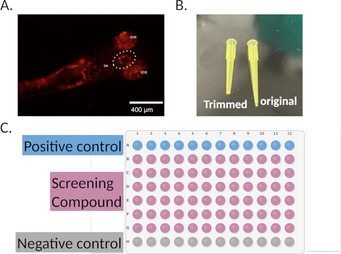
Figure 1: Transgenic screening, larval embedding, and plate design. (A) Fluorescence image (mCherry channel, 4× objective) of a transgenic zebrafish larva expressing nitroreductase (NTR) in dopaminergic (DA) neurons, showing DA neuron clusters in the ventral diencephalon between the eyes. (B) Modified P200 pipette tips trimmed to approximately 1.5 mm openings, used for transferring larvae during agarose embedding. (C) Representative 96-well plate layout for high-throughput drug screening, including vehicle control, metronidazole (MTZ)-treated wells, and screening compound conditions. Please click here to view a larger version of this figure.

3. Chemogenetic Ablation and Fluorescence Imaging

1. Prepare agarose embedding medium
   1. On the day of embedding at 4 dpf, prepare 1.2% low melting point agarose (LMA) in Milli-Q water.
   2. Heat the agarose solution in a microwave in short 5–10 s intervals, swirling gently between intervals, until the agarose is fully dissolved and the solution is clear. Avoid boiling over or prolonged heating, which can alter the final agarose concentration through evaporation.
   3. Aliquot the agarose into 1.5 mL microcentrifuge tubes.
   4. Melt aliquots at 70°C and equilibrate them in a 42°C heat block before use.
   5. Add 20 µL of tricaine stock solution (4 mg/mL) to each agarose aliquot to achieve a working concentration of approximately 40 µg/mL.
   6. Mix tricaine into the molten agarose by gently pipetting up and down 5–10 times using a P200 pipette. Avoid vortexing or introducing bubbles, as bubbles can interfere with larval positioning and imaging.
2. Anesthetize and embed larvae
   1. Add tricaine stock solution to the Petri dish containing 4 dpf larvae to achieve a final concentration of 160 µg/mL.
   2. Incubate larvae in tricaine for approximately 5 min, or until they show loss of spontaneous swimming and no response to gentle touch with a probe. Proceed with embedding only after this anesthesia endpoint is reached.
   3. Trim the distal end of a P200 pipette tip using clean scissors or a sterile blade to create an opening of approximately 1.5 mm. Verify the opening size using a ruler or calibrated scale under a stereomicroscope before use. Discard tips with rough edges or openings that are too narrow for larvae to pass through without contact (Figure 1B).
   4. Aspirate a single larva in minimal liquid using the modified pipette tip.
   5. Submerge the pipette tip into the agarose aliquot.
   6. Dispense 40 µL of agarose containing one larva into one well of a flat-bottom 96-well plate. Use the same agarose volume for all wells within an experiment. If a different plate type is used, optimize the agarose volume before beginning the experiment and maintain the selected volume across all wells.
      ​NOTE: Use flat-bottom plates to ensure consistent imaging. Optimize agarose volume based on plate geometry.
3. Orient and embed larvae
   1. Place the plate under a stereomicroscope (dissection microscope).
   2. Use fine-tipped forceps or a 0.25 mm probe to orient the larva such that the ventral diencephalon faces the objective.
   3. Position larvae dorsal side down for inverted microscopes or dorsal side up for upright microscopes.
   4. Complete orientation within 1–2 min before agarose solidifies.
   5. Embed one larva per well according to a predefined 96-well plate map. Reserve row A for vehicle controls, row H for MTZ-only controls, and assign rows B–G to candidate compound conditions or dose-response groups. Randomize compound placement within rows B–G when possible to reduce positional bias. Use the same plate map for baseline and post-treatment imaging.
   6. After agarose solidification, add BEW without tricaine to each well to bring the final well volume to exactly 200 µL. Use the same final volume for all wells within the plate to maintain consistent diffusion and treatment exposure.
4. Prepare MTZ treatment solutions
   1. Prepare MTZ working solutions in BEW supplemented with 1% DMSO and 200 µM PTU. Add MTZ powder to the solution and vortex until no visible particles remain. Mix on a rocker or tube rotator protected from light for 15–30 min at room temperature. Confirm that the solution is clear and free of visible precipitate before use.
   2. Prepare concentrations of 3, 4.5, and 9 mM for dose-response optimization.
   3. Prepare a vehicle control containing 1% DMSO in BEW with 200 µM PTU.
   4. Prepare only the validated MTZ concentration for routine screening after optimization.
      CAUTION: MTZ is light-sensitive. Prepare solutions fresh for each experiment, protect from light using foil, and do not reuse leftover solutions.
      ​NOTE: Maintain identical final DMSO concentrations across all treatment and control groups. Do not substitute alternative MTZ formulations.
5. Acquire pre-treatment fluorescence images
   1. At 4 dpf, after embedding, acquire baseline fluorescence images using a fluorescence microscope with a 20× objective (Figure 2).
   2. Image each well using the mCherry channel (excitation ~587 nm, emission ~610 nm).
   3. Use identical imaging settings for all wells within an experiment. Set exposure time, illumination intensity, and detector gain using a vehicle control larva so that the brightest DA neuron pixels reach approximately 70%–80% of the detector dynamic range without saturation. Record the final exposure time, illumination intensity, detector gain, objective, and acquisition profile, and maintain these settings for all baseline and post-treatment images.
   4. Acquire all images within a single session when possible to minimize variability in lamp intensity or detector sensitivity across time points. For systems with automated stage control, use multiposition acquisition to maintain identical coordinates across imaging sessions.
   5. Save the acquisition profile for reuse during post-treatment imaging (Step 3.7) and in subsequent experiments.
      ​NOTE: A 20× objective provides a balance between field of view and resolution for imaging the diencephalic DA neuron cluster.
6. Apply MTZ treatment after baseline imaging
   1. Immediately after baseline imaging at 4 dpf, add MTZ-containing solution or vehicle solution directly to each well to bring the final well volume to 200 µL.
   2. For compound-screening experiments, add candidate compounds together with MTZ at this step so that larvae are exposed to MTZ ± compound during the same 24 h treatment period.
   3. Incubate plates at 28.5°C under a 14 h light:10 h dark cycle for 24 h, from 4 dpf to 5 dpf.
   4. Avoid disturbing the plates during incubation.
      NOTE: For dose-response experiments, evaluate additional incubation times (e.g., 12 and 48 h) to optimize treatment conditions.
      ​PAUSE POINT: Plates can be maintained under incubation conditions for the defined treatment duration before proceeding to imaging.
7. Acquire post-treatment fluorescence images
   1. At 5 dpf, acquire post-treatment images using the identical microscope settings used for baseline imaging at 4 dpf, including exposure time, illumination intensity, detector gain, objective, and acquisition profile (Figure 2).
   2. Do not adjust exposure time, detector gain, illumination intensity, focus, objective, or acquisition settings between wells or between pre-treatment and post-treatment imaging sessions.
   3. If the microscope was powered off between sessions, reload the saved acquisition profile and verify all settings against the recorded parameters before imaging.
   4. Image wells in the same order used during baseline imaging when possible and acquire all post-treatment images within the same imaging session.
   5. This paired pre-treatment and post-treatment imaging design controls for inter-individual variability in baseline DA neuron fluorescence and ensures that changes in signal are attributable to treatment rather than acquisition differences.

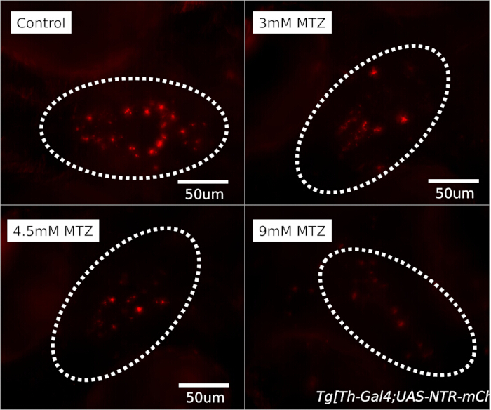
Figure 2: Dose-dependent reduction in DA neuron fluorescence following metronidazole treatment. Representative fluorescence images (mCherry channel, 20× objective) of transgenic zebrafish larvae showing diencephalic DA neurons after 24 h treatment with varying concentrations of MTZ. Fluorescence intensity decreases in a dose-dependent manner, indicating successful chemogenetic ablation of NTR-expressing neurons. Scale bar = 50 µm. Please click here to view a larger version of this figure.

4. High-Throughput Plate-Based Drug Screening

1. Generate and screen transgenic larvae
   1. Generate a new cohort of homozygous transgenic larvae.
   2. Collect embryos and raise them in BEW.
   3. Treat embryos with 200 µM PTU at 24–36 h post-fertilization (hpf) as described in Step 2.3.
   4. At 3 dpf, screen larvae using the mCherry channel with fixed microscope settings for all larvae within the experiment. Set exposure time, detector gain, and illumination intensity using a known positive larva to clearly detect DA neuron fluorescence without saturation, then keep these settings unchanged during screening.
   5. Classify larvae as positive if clear mCherry fluorescence is visible in the expected DA neuron clusters of the ventral diencephalon under fixed screening settings. Discard larvae with no signal above background in this region or with weak, diffuse, or ectopic fluorescence.
2. Embed larvae and acquire baseline images
   1. At 4 dpf, embed larvae in a 96-well plate as described in Steps 3.2–3.3, using one larva per well.
   2. Acquire pre-treatment baseline fluorescence images as described in Step 3.5.
3. Apply MTZ and candidate compounds
   1. After acquiring baseline fluorescence images at 4 dpf, add treatment solutions directly to wells according to the plate map (Figure 1C).
   2. For vehicle control wells, add BEW containing the same final DMSO concentration used in compound-treated wells.
   3. For MTZ-only control wells, add MTZ solution without candidate compound.
   4. For compound-screening wells, add MTZ and candidate compound together so that larvae are exposed to both during the same 24 h treatment period.
   5. For initial screening, use a single compound concentration, such as 10 µM, unless compound-specific solubility, toxicity, or prior dose-response data indicate that a different concentration should be used.
   6. Adjust each well to a final volume of 200 µL. Maintain identical final DMSO concentrations across all wells, including vehicle control, MTZ-only control, and MTZ plus compound wells.
   7. Incubate plates at 28.5°C under a 14 h light:10 h dark cycle for 24 h, from 4 dpf to 5 dpf.
      ​NOTE: This protocol does not include MTZ removal or washout before compound exposure. Candidate compounds are applied concurrently with MTZ immediately after baseline imaging.
4. Acquire post-treatment images and calculate fluorescence retention
   1. At 5 dpf, acquire post-treatment fluorescence images using the identical acquisition settings used for baseline imaging at 4 dpf.
   2. Image wells in the same order used during baseline imaging whenever possible.
   3. Calculate fluorescence retention for each larva as:
      
   4. Normalize fluorescence retention values to the mean vehicle control value from the same plate.
   5. Identify candidate protective compounds as those with fluorescence retention values significantly greater than the MTZ-only control.
5. Identify hit compounds
   1. Identify hit compounds as those with fluorescence retention ratios significantly greater than the negative control (MTZ-only).
   2. Perform statistical analysis using Welch’s t-test to compare MTZ-only controls with MTZ plus compound treatment groups.
   3. Validate hit compounds using independent biological replicates and dose-response assays. Confirm hits as compounds that reproducibly increase fluorescence retention relative to the MTZ-only control, with p < 0.05 and no visible larval toxicity or abnormal morphology.
   4. Advance validated hits to secondary assays such as locomotor behavioral analysis, dose-response validation, or independent biological replicate testing.
      NOTE: For compound library screens, calculate the Z-factor for each plate using positive and negative controls. A Z-factor > 0.5 indicates a robust assay suitable for hit identification.

5. Locomotor Behavioral Assessment

1. Assign larvae to treatment groups
   1. At 4 dpf, allocate larvae from each genotype into three treatment groups with at least 10 larvae per group: BEW only, DMSO vehicle control, and MTZ treatment.
   2. Assign groups as follows: (1) BEW only (untreated baseline), (2) 1% DMSO vehicle control, and (3) optimized MTZ concentration (4.5 mM in 1% DMSO/BEW with 200 µM PTU).
   3. Include AB wild-type larvae treated with vehicle or MTZ under identical conditions. Confirm NTR-dependent effects if MTZ reduces locomotion in Tg(th:Gal4; UAS:NTR-mCherry) larvae but not in AB wild-type larvae.
2. Perform treatment and plate larvae
   1. Treat larvae for 24 h at 28.5°C using the conditions defined in Step 5.1.2: BEW only, 1% DMSO vehicle control, or 4.5 mM MTZ in 1% DMSO/BEW with 200 µM PTU.
   2. Transfer five larvae into each well of a 6-well plate containing 2.5 mL fresh BEW using a wide-bore transfer pipette. Minimize carryover volume and handle larvae gently to avoid stress or injury.
      ​NOTE: Using five larvae per well balances data yield and minimizes overcrowding. Higher densities increase path crossings and introduce tracking errors in behavioral analysis.
3. Set up illumination conditions
   1. Place the 6-well plate on a white LED light pad with uniform diffused illumination maintained at 25°C–28°C. Use the same light pad, brightness setting, and plate position for all recordings within an experiment (Figure 3A).
   2. Illuminate the plate from both below and above using diffused light sources to minimize shadows, glare, and reflections.
4. Configure video recording setup
   1. Mount a high-resolution camera in a fixed top-down orientation above the plate using a stable support (e.g., tripod or arm mount) (Figure 3B).
   2. Place a ruler adjacent to the plate within the field of view for spatial calibration.
   3. Ensure that the camera is perpendicular to the plate surface to minimize parallax distortion.
5. Record locomotor activity
   1. Conduct recordings during the light phase of the 14 h light:10 h dark cycle to minimize circadian variability.
   2. Allow larvae to acclimate for 1 h before recording.
   3. Record locomotor activity for 60 min.
   4. Do not disturb the setup during recording.
      ​NOTE: Perform recordings at the same time of day across experiments to minimize circadian variability.
6. Configure behavioral tracking software
   1. Import the recorded video into EthoVision XT (behavioral tracking software) (Figure 3C).
   2. Configure the following settings: 6 arenas, 5 subjects per arena, center-point detection, distance in millimeters, and time in seconds.
   3. Calibrate the spatial scale using the ruler present in the video frame.
   4. Define arena boundaries for each well, ensuring that each arena fully encompasses the well interior without extending beyond the well edges.
7. Optimize detection settings
   1. Generate a reference image using the software interface (Detection Settings → Reference Image → Start Learning).
   2. Adjust the detection threshold to ensure accurate tracking of all larvae without false detections.
   3. Run a short test acquisition (~2 min).
   4. Inspect tracked paths visually before proceeding to full analysis. Confirm that all larvae are detected and that bubbles, debris, reflections, or well edges are not falsely identified as larvae.
      ​NOTE: Common artifacts include edge tracking caused by oversized arenas, false detections from bubbles or debris, and loss of tracking during prolonged inactivity.
   5. Exclude wells from analysis if persistent tracking failure, excessive path crossing, visible debris or bubbles, dead larvae, abnormal morphology, or larvae trapped at the well edge prevents reliable quantification.
   6. Apply the same exclusion criteria to all treatment groups before statistical analysis.
8. Perform full analysis and export data
   1. Run the full acquisition.
   2. Generate track visualizations and heatmaps (Analysis → Results → Tracks and Heatmaps).
   3. Export the raw data spreadsheet containing per-subject metrics, including total distance traveled (mm), mean velocity (mm/s), and number of movement bouts.
   4. Use total distance traveled over 60 min as the primary locomotor endpoint (Figure 3D).

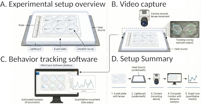
Figure 3: Locomotor behavioral recording setup and analysis workflow. (A) Experimental setup showing a 6-well plate containing zebrafish larvae positioned on a light pad with a ruler for spatial calibration and a temperature-controlled heat source for maintaining experimental conditions. (B) Video acquisition setup with a top-down camera used to record larval movement, with representative tracking overlay. (C) Behavioral tracking performed using EthoVision XT (behavioral tracking software), showing automated detection and tracking of larval movement. (D) Workflow summary outlining the steps from video acquisition to quantitative analysis of locomotor behavior. Please click here to view a larger version of this figure.

6. Data Analysis

1. Prepare images for analysis
   1. Open pre-treatment and post-treatment image pairs in Fiji (ImageJ, image analysis software).
   2. If images are acquired as Z-stacks, generate maximum intensity projections (Image → Stacks → Z Project → Max Intensity).
   3. Adjust Brightness/Contrast using identical fixed display settings for all images within a dataset. Do not use auto-scaling for quantitative measurements, and perform fluorescence quantification on the original unadjusted images.
2. Define regions of interest (ROI)
   1. Use the polygon selection tool to draw an ROI around the diencephalic DA neuron cluster in the pre-treatment image. Define the ROI boundary using anatomical landmarks visible in the fluorescence image, including the medial edges of the eyes and the ventral midline of the diencephalon (Figure 2). Ensure that the ROI encompasses the entire DA neuron cluster without extending into adjacent fluorescent structures. For consistency across operators, save a representative ROI template and distribute it to all team members as a spatial reference.
   2. Press “t” to add the ROI to the ROI Manager.
   3. Align pre-treatment and post-treatment images using anatomical landmarks, including the eyes and ventral diencephalon, before applying the ROI. Apply the same ROI to the matched post-treatment image only after confirming alignment.
   4. Save all ROIs for each plate to enable reproducibility and re-analysis.
3. Quantify fluorescence intensity
   1. Configure measurement settings (Analyze → Set Measurements) and select “Area” and “Mean gray value.”
   2. Measure each image (Analyze → Measure).
   3. Measure background fluorescence from an adjacent non-neuronal region within the same image and subtract it from the DA neuron ROI measurement. Calculate background-corrected integrated density as: corrected IntDen = IntDenROI − (areaROI × mean background).
   4. Calculate the fluorescence retention ratio for each larva as IntDen(post-treatment) / IntDen(pre-treatment).
   5. Normalize fluorescence retention ratios to the mean vehicle control value from the same plate. Calculate the vehicle control mean separately for each plate before comparing treatment groups¹⁹.
      ​NOTE: For higher-throughput analysis, perform the same quantification using CellProfiler (image analysis software) with automated ROI detection²⁰.
4. Perform pairwise statistical analysis
   1. For comparisons between one treatment group and one control group, perform an unpaired two-tailed Welch’s t-test, which does not assume equal variance between groups.
   2. Use this test when variance differs between groups.
5. Perform multi-group statistical analysis
   1. Perform one-way ANOVA for experiments involving multiple treatment groups.
   2. Apply Dunnett’s post hoc test to compare each treatment group with the control group using GraphPad Prism or equivalent statistical software.
6. Report statistical results
   1. Set the significance threshold at α = 0.05.
   2. Report exact p-values rather than categorical thresholds.
   3. Present data as mean ± standard error of the mean (SEM) with individual data points overlaid as scatter plots using GraphPad Prism or equivalent graphing software.
   4. Report sample size (n), statistical test, test statistic, degrees of freedom, and exact p-value in the figure legends. For large datasets, include full statistical outputs in a supplementary table.
      NOTE: For screening assays, calculate the Z-factor for each plate as Z = 1 − [3(σ_p + σ_n)/|µ_p − µ_n|], where σ_p and µ_p are the standard deviation and mean of the vehicle control group, and σ_n and µ_n are the standard deviation and mean of the MTZ-only control group. A Z-factor > 0.5 is considered acceptable for screening.

Results

MTZ Treatment Produces Dose-Dependent Dopaminergic Neuron Loss and Locomotor Impairment

To determine the optimal parameters for MTZ-mediated ablation of DA neurons, fluorescence intensity, used as a proxy for DA neuron survival, and locomotor distance were evaluated across MTZ concentrations of 3, 4.5, and 9 mM following 24 h treatment. Each treatment group consisted of n = 10 individual Tg(th:Gal4; UAS:NTR-mCherry) larvae with a matched vehicle control group (1% DMSO in BEW w...

Discussion

This protocol offers a scalable, in vivo pipeline for quantifying DA neuronal loss and screening neuroprotective compounds using the NTR–MTZ chemogenetic system in transgenic zebrafish. The standardized, plate-based workflow was specifically developed for undergraduate research teams, where operator turnover is high and investigator experience varies between academic terms. Each step of the workflow has been structured to prioritize reproducibility and ease of training, enabling consistent execution across multiple...

Materials

List of materials used in this article

Name	Company	Catalog Number	Comments
Adult zebrafish diet, 0.5 mm pellets	Zeigler	AH271	Used for feeding adult zebrafish during routine husbandry
Agarose, low melting point (LMA)	Sigma-Aldrich	A9414-10G	Used for embedding larvae in wells for stable positioning during imaging
Aluminum foil	ULINE	S-20197	Used to protect light-sensitive reagents such as MTZ during preparation and incubation
CellProfiler	Broad Institute	RRID: SCR_007358	Used for optional automated fluorescence image analysis
Conical tubes, 15 mL	Corning	352097	Used for reagent preparation and sample handling
Conical tubes, 50 mL	Corning	352070	Used for reagent preparation and solution storage
Crossing tanks (1.0 L)	Aquaneering	ZHCT100	Used for controlled zebrafish breeding and embryo collection
Danio rerio (AB wild type)	—	—	Non-transgenic control line used to validate specificity of nitroreductase-dependent effects
Danio rerio (Tg(th:Gal4; UAS:NTR-mCherry))	—	—	Transgenic zebrafish line expressing nitroreductase-mCherry in dopaminergic neurons for targeted chemogenetic ablation
Dimethyl sulfoxide (DMSO), anhydrous (≥99.9%)	Sigma-Aldrich	472301-500ML	Solvent for PTU, MTZ, and screening compounds
EthoVision XT	Noldus	RRID: SCR_000441	Behavioral tracking software used to quantify larval locomotion
Fiji (ImageJ)	NIH	RRID: SCR_003070	Image analysis software used for fluorescence quantification
Fine-tipped forceps or 0.25 mm probe	World Precision Instruments	WPI0118	Used to orient larvae during agarose embedding
Fluorescence microscope	Zeiss	11845460	Used to image dopaminergic neurons via mCherry fluorescence
Gemma Micro 150 ZF (juvenile diet, 100–200 μm)	Skretting	10818945	Used to feed juvenile zebrafish
Gemma Micro 75 ZF (larval diet, 50–100 μm)	Skretting	10818935	Used to feed larval zebrafish
GraphPad Prism	GraphPad	RRID: SCR_002798	Statistical analysis software used for data analysis and plotting
Heat block (42°C and 70°C capable)	Thermo Fisher	88870001	Used to melt and maintain agarose at controlled temperatures
High-resolution camera (top-down mount compatible)	Basler	88-327	Used to record larval locomotor activity
Hydrochloric acid (HCl), 0.1 M	Fisher Scientific	SA48-500	Used to adjust pH during tricaine preparation
Incubator (28.5°C, 14 h light:10 h dark photoperiod)	Millipore	Z763314	Maintains controlled environmental conditions for zebrafish development
Instant Ocean sea salt	Instant Ocean	SS15-10	Used to prepare blue egg water (BEW)
Light diffuser sheet (or equivalent)	Edmund Optics	27-103	Used to provide uniform lighting and minimize glare during behavioral recording
Light pad	Lightcraft	LC2004LED	Provides bottom illumination during locomotor tracking
Metronidazole (MTZ)	Sigma-Aldrich	M3761-100G	Used for chemogenetic ablation of dopaminergic neurons
Methylene blue, 1% aqueous solution	Sigma-Aldrich	M9140	Added to BEW to prevent microbial growth in embryos
Microcentrifuge tubes, 1.5 mL	Eppendorf	22363204	Used for reagent aliquoting and storage
Micropipette, P200	Gilson	FP10005S	Used for handling larvae and preparing solutions
Petri dishes, 100 mm	Corning	CLS430167	Used for embryo collection and incubation
Pipette tips, 200 μL	RAININ	30389188	Used with micropipettes for liquid handling and larval transfer
Sodium chloride (NaCl), ≥99.0%	Sigma-Aldrich	S9888-500G	Used for preparing buffer and aqueous solutions
Sodium hydroxide (NaOH), 0.1 M	Fisher Scientific	SS256-500	Used to adjust pH during tricaine preparation
Stereomicroscope	Nikon	SMZ-745	Used for larval manipulation and orientation during embedding
Temperature-controlled heat mat (25°C–28°C)	Vivosun	V-SHMDT	Maintains stable temperature during behavioral recording
Tricaine methanesulfonate (MS-222)	Sigma-Aldrich	E10521-10G	Used as an anesthetic for zebrafish larvae
Tris base	Fisher Scientific	BP152-1	Used in preparation of buffered tricaine solution
Water purification system	Millipore	ZIQ7003T0	Used to generate deionized water for solution preparation
Zebrafish holding tanks	Aquaneering	ZS560	Used for maintaining adult zebrafish populations
1-Phenyl-2-thiourea (PTU)	Sigma-Aldrich	P7629-10G	Used to inhibit melanogenesis and maintain optical transparency
6-well plate, flat bottom	Corning	07-200-83	Used for locomotor behavioral assays
96-well plate, flat bottom	Greiner Bio-One	655096	Used for high-throughput imaging and screening assays