Constructing Legal Knowledge Graphs and Tracing Bias in Medical Artificial Intelligence Based on Graph Neural Networks

Summary

Addressing legal text fragmentation and medical artificial intelligence (AI) bias-tracing issues, this study constructs a legal knowledge graph and employs relation-aware graph convolution for semantic alignment. It identifies biased sources via gradient-based backpropagation, with favorable experimental metrics to support a compliant medical AI application.

Abstract

In medical artificial intelligence (AI) legal compliance analysis, this paper addresses the ambiguity in liability determination caused by the semantic fragmentation of multi-source heterogeneous legal texts and difficulties in tracing algorithmic biases. It constructs a knowledge graph construction and bias propagation path detection method based on graph neural networks. Four types of heterogeneous nodes—legal clauses, medical behaviors, algorithm modules, and responsible parties—are structured and encoded, and a directed graph is constructed based on four types of legal semantic relationships: "violation", "basis", "trigger", and "attribution". Next, a relation-aware graph convolutional network, combined with edge-type-specific weights and an attention mechanism, is used to achieve multi-layer feature alignment for cross-modal legal semantics. Then, gradient-based backpropagation is used to identify edges that significantly contribute to bias, construct a bias-propagation subgraph, and use community discovery to locate root-node clusters. Finally, real-time decision flows are mapped to temporary nodes, compliance is verified by embedding similarity, and the dynamics of key edge weights are monitored to warn of systemic bias accumulation. Experiments show that, in terms of semantic alignment accuracy, the proposed method achieves an average entity alignment accuracy of at least 0.92 and an average relation preservation completeness of at least 0.88 across different knowledge graph density gradients. Regarding bias localization capability, the root node recall rate reaches 0.95±±0.02, and the propagation path precision reaches 0.93±±0.03. This research, to a certain extent, achieves a deep coupling between legal logic and algorithmic behavior, providing an explainable and verifiable compliance support system for the trustworthy deployment of medical AI.

Introduction

The profound involvement of medical AI in diagnosis and treatment support, resource allocation, and risk assessment has tied its decision-making to the assumption of legal responsibility^1,2. The legal norms are highly structured but semantically distributed, and the behaviour of AI systems can be black-boxed, without a semantically alignable and traceable interface between the two³. In this context, developing a common representation framework that captures legal causal chains within algorithmic behavioral sequences has emerged as a necessary enabler to realize fine-grained attribution of responsibility and dynamic compliance^4,5. This study is not only related to the legal testing of technology systems, but also involves the deep maintenance of medical fairness, algorithmic fairness, and institutional trust, and thus has great theoretical significance and practical urgency.

The fundamental issue in legal conformance analysis of medical AI today is the lack of a computable connective structure between legal semantics and algorithmic behavior^6,7. Legal documents are available as plain text, and the relations between paragraphs are interwoven with dependencies, conflicts, and exceptions, causing problems when splitting them into logical units that can be interpreted by machines^8,9. Although the AI system’s decision-making is encapsulated in a data-driven black box, and none of its output variations can be traced to specific breaches in legal duties or nodes for apportionment of liability^10,11. Such disconnection (for example, training data bias, model design flaws, or the semantic interpretation of legal norms) cannot be experimentally isolated to identify the source of bias or to clarify legal duties for developers, deployers, or users^12,13. Even more problematic, existing compliance procedures only check whether a final output meets a fixed specification, without considering the propagation path or amplification of bias in the "law-technology" network of interactions^14,15. When medical AI is subject to multiple legal provisions simultaneously, and the system produces a chain of errors due to misinterpretation of one clause, conventional approaches cannot trace how the error diffuses through other related provisions and then reaches the liability^16,17. In addition, there is a lack of a dynamic correlation mechanism between the real-time decision flow and the existing knowledge graph of law, resulting in delayed compliance evaluation during system operation, thus preventing a proactive monitoring of the trend of accumulation of bias^18,19. These issues together lead to uncertainty in liability determination, fragile attribution, and delayed regulatory intervention, which significantly inhibit the trustworthy deployment of high-risk healthcare AI systems and the application of legal accountability.

Above all, traditional research studies legal texts in a structured form and builds knowledge bases of specific domains with ontologies or rules in order to support compliance questions and answers or risk notification^20,21. Although these approaches can capture representations of some legal concepts, they tend to presuppose the law's internal logic as coherent and static, making it difficult to deal with inter-jurisdictional inconsistencies, exceptions, or vague formulations. Subsequent work introduced natural language processing technology, using pre-trained language models to extract legal entities and relationships, improving the breadth of knowledge extraction coverage^22,23, but still remains at a shallow semantic level, failing to establish a mapping interface between legal and technical behaviors. In terms of algorithmic bias governance, research has mostly focused on the design of fairness constraints^24,25, and its evaluation indicators are usually based on demographic variables, lacking alignment with legal attribution principles. Even some studies have attempted to encode legal rules as constraints and embed them into model training^26,27, but due to the rigidity and coarse granularity of rule expression, they are difficult to adapt to complex clinical situations. In general, existing work treats legal compliance as an external verification task rather than an intrinsic computable attribute of the system architecture. This results in legal logic and algorithmic logic operating in parallel, failing to support joint reasoning and dynamic intervention on bias propagation paths.

In recent years, graph neural networks have been gradually introduced into the medical field due to their explicit modeling capabilities of relational structures^28,29. Some studies utilize heterogeneous graphs to integrate case law, legal provisions, and party information, supporting case recommendations or sentencing predictions through node embeddings^30,31, thereby verifying the effectiveness of graph structures in capturing legal connections. Other works abstract algorithmic components as graph nodes, using edges to represent data flows or call relationships for tracking error propagation^32,33. These explorations demonstrate that graph structures can serve as a common carrier of legal and technological elements. However, existing graph models generally suffer from three limitations: first, they are limited to a single type of edge relationship, failing to distinguish between normative, causal, and attributional differences in legal semantics; second, the feature aggregation process ignores the semantic weights of edge types, leading to different legal logic paths being treated equally; and third, they lack a differentiable tracking mechanism for bias propagation, making it impossible to locate high-contribution edges and reconstruct responsibility paths. This paper constructs a relation-aware graph convolutional network that addresses the problem of semantic heterogeneity fusion by assigning a dedicated transformation matrix to each type of legal semantic edge and introducing an attention mechanism to dynamically adjust cross-type information flow. Furthermore, by combining gradient backpropagation and subgraph extraction, it enables an interpretable leap from macro-level compliance judgment to micro-level bias tracing, overcoming the bottleneck of traditional graph models that only support static reasoning.

Beyond the medical domain, recent advances in graph-based and evolutionary methods have demonstrated broad applicability to structured knowledge processing. For instance, Xue et al. proposed a multilayer hybrid genetic programming approach for adaptive similarity feature construction in ontology matching, achieving robust alignment across heterogeneous knowledge graphs³⁴. Cheng et al. provided a comprehensive survey of graph convolutional network applications in image restoration, systematically categorizing methods for denoising, super-resolution, and deblurring³⁵. Li et al. presented a thorough survey on evolutionary deep learning from the perspective of automated machine learning, covering principles, algorithms, applications, and open challenges³⁶. Ma et al. developed a fuzzy neural architecture search framework for defect recognition under uncertainty, demonstrating the effectiveness of evolutionary search in handling ambiguous data³⁷. These studies highlight the potential of integrating graph-structured representations and evolutionary optimization for complex decision-making tasks.

The core objective of this paper is to establish an end-to-end interpretable framework for legal compliance analysis of medical AI, with innovations at three levels. At the knowledge representation level, it is the first to model legal clauses, medical practices, algorithm modules, and responsible parties as four types of heterogeneous nodes. Based on legal practice, it extracts four types of directed relationships: "violation", "basis", "trigger", and "attribution", constructing a directed knowledge graph with legal causal logic, providing a structured semantic foundation for compliance analysis. At the source tracing of bias, it suggests a gradient-sensitivity-based edge contribution quantification method. By backpropagation, it finds the set of edges that maximizes the output bias, then applies a community discovery algorithm to cluster high-contribution nodes, turning "black-box bias" into "white-box responsibility clusters", which makes attribution based on an operable chain of evidence. At the level of real-time dynamic monitoring, it develops a temporary decision-node embedding mechanism that maps real-time AI outputs into the knowledge graph space. Based on the comparison of embedding proximity, it quantifies the degree of norm deviation and monitors the weight change of those essential legal-technical edges, so as to signal the accumulation of systemic bias. This paradigm addresses both semantic fragmentation and traceability conundrums and metamorphoses legal compliance from ex post verification into ex ante governance, offering a scalable technical avenue for the transparency of responsibility in high-risk AI systems.

Protocol

Construction of graph neural network for medical AI legal knowledge graph

As shown in Figure 1, the proposed framework comprises three main modules. The input layer integrates multi‑source data into a heterogeneous graph via multimodal entity encoding and directed edge modeling. The relation‑aware GCN layer then performs cross‑modal semantic alignment through type‑specific weights and attention, producing unified node embeddings. Finally, these embeddings support bias tracing (via gradient backpropagation and community detection) and dynamic compliance monitoring (via real‑time node mapping and edge‑weight tracking), with the output delivering interpretable attribution evidence and risk alerts for regulators.

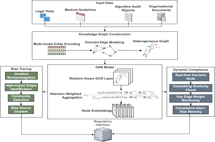
Figure 1: Legal knowledge graph and bias tracing architecture for medical AI. This diagram illustrates the overall workflow of the proposed framework. The input layer fuses multi‑source heterogeneous data (legal texts, clinical guidelines, algorithm audit reports), which are encoded into four entity types (legal clauses, medical behaviors, algorithm modules, responsible parties) and connected by four directed legal‑semantic relations (violation, basis, trigger, attribution). The relation‑aware GCN layer performs cross‑modal semantic alignment via type‑specific weights and attention. The bias tracing module uses gradient backpropagation to identify high‑contribution edges, then applies community detection to locate root‑node clusters. The dynamic compliance monitor maps real‑time decisions to temporary nodes, evaluates embedding similarity against legal clauses, and tracks edge weight evolution for early warning. Outputs include interpretable attribution evidence and risk alerts. Please click here to view a larger version of this figure.

Heterogeneous graph structured coding of legal entities and relationships

Four fundamental entities are consistently derived from medical AI regulatory laws, clinical practice guidelines, and algorithm audit reports: legal clauses, medical procedures, algorithm modules, and accountable entities. A separate feature representation learning model is proposed for each type of entity to be semantically distinguishable. The legal clause nodes are organized to contain the number of the legal clause, and this is used as a unique ID (identifier) for the legal clause. At the same time, a penalty severity quantification index is defined to indicate the level of legal responsibility associated with the clause, and consequently, a feature vector is established.

（1）

c_i is the entry number, Emb(·) represents the low-dimensional embedding mapping, and [·;·] represents the vector concatenation operation. This representation preserves both the formal structure and the severity of punishment of the legal text, supporting cross-statement reasoning.

Medical behavior nodes are standardized and encoded based on a clinical operation classification system, extracting their risk level r_j ∈ {1,2,3} and the set of applicable scenario labels s_j ⊂ S, where S is the complete set of predefined scenario categories. Multi-hot encoding is used to process the label set, and it is concatenated with the risk level embedding to form an initial representation:

（2）

This strategy ensures that different types of medical behaviors have measurable distance relationships in the vector space, supporting cross-scenario comparisons. The text embedding function Emb(·) is implemented using the pre-trained Chinese legal language model Lawformer (pretrained on a large-scale Chinese legal corpus), with the output dimension fixed at 768.

Based on the logical dependencies and legal constraints between entities, four types of directed semantic relationships are established: "violation", "basis", "trigger", and "attribution", each corresponding to different legal causal patterns. Each edge e_ij ⊂ E is assigned a type of label t_ij ⊂ T = {violate, base, trigger, attribute} for subsequent message transmission for relationship awareness. Edge construction strictly follows the domain rule matching mechanism: when a medical behavior deviates from the normative requirements, a "violation" edge is established pointing from the behavior node to the relevant legal clause; when the legal clause serves as the technical compliance basis for an operation, a "basis" edge is established; if the output of the algorithm module directly triggers the execution of a specific medical behavior, a "trigger" edge is connected; the attribution of responsibility relationship is established based on the organization's responsibility documents and audit conclusions, establishing an "attribution" edge between the responsible party and the violation or algorithm defect.

After all nodes are initialized, a heterogeneous graph (V, E, H⁰) is formed, where V is the set of nodes, E is the set of directed edges with type labels, and H⁰ is the initial feature matrix. To enhance the semantic discriminative ability of the graph structure, the node features are normalized:

（3）

μ_k and σ_k are the mean and standard deviation of the k-th node feature on the training set, respectively, and ∈ is a small constant to prevent division by zero. Normalization ensures that multi-source heterogeneous features participate in graph convolution operations on a uniform scale, preventing numerical dominance effects from interfering with semantic learning. The resulting structured graph model fully carries the relational topology of the four-dimensional elements of law, behavior, technology, and responsibility in the medical AI system, providing a computable graph basis for subsequent bias propagation analysis.

Graph convolution alignment enhancement for cross-modal legal semantics

A relation-aware graph convolutional network^38,39, which extends the Relational Graph Convolutional Network (R-GCN) framework, is used to propagate features across multiple layers of the initial heterogeneous graph. While R-GCN introduces per-relation transformation matrices for general relational data, our approach further incorporates a learnable attention mechanism to dynamically weight neighbor contributions and defines four specific legal-semantic relation types (violation, basis, trigger, attribution) tailored to medical AI compliance analysis.. Each layer's operation independently parameterizes the transformation process based on the semantic type of the edges. For any target node, its neighborhood information is grouped and aggregated by the types of connecting edges. Each type of relation is equipped with a dedicated linear transformation matrix to differentiate the features transmitted along different legal semantic paths^40,41. If the edge between the legal clause node and the medical behavior node is of "base" type, when the legal clause node receives a message from a medical behavior node, it applies the corresponding weight matrix to map the features of the neighbor spatially. In the same way, when a medical behavior node sends an output via the edge integration scheme module node "trigger" to an algorithm module, the parameter matrix triggered, associated with this relation, and performs feature transformation. This mimics the fluidity of different types of legal logic, realizing/informing different logic layers to maintain semantic independence during information flow without cross-modal noise. The aggregation is defined as follows:

（4）

m_i^(l) represents the comprehensive information collected by node i in layer l, N_i^l is its neighbor set under relation r, W_r is the linear transformation matrix, and h_j^(l−1) is the embedding representation of the neighbor node in the previous layer.

A learnable attention mechanism is introduced during message aggregation to dynamically adjust the influence intensity of different neighbor nodes on the target node representation update^42,43. The attention coefficient is generated based on the dual factors of node attribute similarity and legal importance, without relying on fixed prior weights. For legal clause nodes, when receiving neighboring medical behavior features, the attention score is calculated based on the quantified value of the penalty intensity associated with the latter; when the algorithm module node fuses medical behavior information, it focuses on neighbors with higher operational risk levels. The attention weight is calculated in the following way:

（5）

α_ij is the attention coefficient of node j to node i, and a is the learnable attention vector. This model allows for the automatic identification of high-risk or high-constraint connected paths during end-to-end training, assigning them higher attention. The final updated node embedding is determined by weighted messages and residual connections.

（6）

σ is the activation function, and residual design mitigates the gradient vanishing problem in deep propagation and guarantees stability in the presence of multiple semantic conflicts. Following L = 3 graph convolutional layers (each with a hidden dimension of 256 and ReLU activation), the embeddings of all nodes seamlessly incorporate cross-modal contextual information and become unified representations with legal semantic discrimination abilities.

Two alternative legal compliance analysis diagrams for the healthcare AI are depicted in Figure 2, with the objective of addressing the visualization of types of legal relationships and routes for bias propagation, indicating potential bias sources of this decision-making. Figure 2A displays the influence of various legal semantic relations, where four relation types are color-coded, and for each type the edges are distinguished by a different color. The thickness of the edge corresponds to the attention weight of that particular relation, i.e. how much this relation contributes to the AI decision. A thick edge indicates essentially a dominant legal relation in the decision and in this case it sufficiently motivated the outcome of the case. Node size is measured by its contribution to violations: larger nodes signify a stronger relationship between the conduct and specific legal clauses, and hence higher potential risk. The above visualization provides a crisp legal semantic layer, which enables us to identify the strongest and riskiest legal paths in AI decision-making. Figure 2B also indicates high-contribution paths (to bias propagation) with emphasis on edges with high contributions, which are bolded and accompanied by dashed lines (e.g. B1-B3) in the decision-making process. Doubling of the width of these edges represents their importance in disseminating systemic bias. Which combinations of legal rules and technical behaviors result in this amplification effect for bias is shown in Figure 2. This analysis not only discloses the path of bias propagation, but also facilitates identifying the origin of bias, based on which compliance auditing and responsibility of the AI tool can be established.

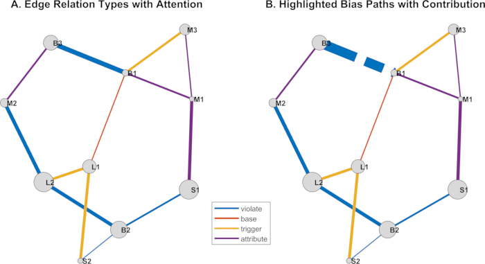
Figure 2: Analysis of legal compliance and bias propagation in healthcare AI (Illustrative Example). (A) Color‑coded legal semantic relations: violation (red), basis (blue), trigger (green), attribution (orange). Edge thickness is proportional to attention weight, indicating the influence of each relation on the AI decision. Node size is proportional to its violation contribution, highlighting risky entities. (B) Bias propagation subgraph: high‑contribution edges are bolded and dashed (e.g., B1‑B3); double‑width edges indicate amplification of systemic bias. This visualization supports identification of dominant legal paths, bias origins, and compliance auditing. No measurement scales or error bars are applicable as this is a schematic illustration. Please click here to view a larger version of this figure.

Subgraph backtracking mechanism for bias propagation path

In this study, "bias" is defined as the systematic deviation of an AI system's output from the clinically and legally expected decision, measured by the discrepancy between the model's predicted risk score and the ground-truth compliance label. The bias signal is quantified as the cross-entropy loss between the algorithm's final output and a binary indicator of compliance (1 for compliant, 0 for non-compliant), aggregated over all decision instances in a batch.

After the graph neural network is trained, its differentiability is used to perform backpropagation analysis on the bias signal in the output layer. Starting from the algorithm decision node that detects anomalies, the gradient magnitude of the loss function with respect to each connecting edge is computed to quantify each edge's contribution to bias formation. This process is implemented through an automatic differentiation framework, backtracking layer by layer along the directed edges in the graph structure to obtain the influence strength of each edge parameter transformation on the final output change. The higher the absolute value of the gradient, the more dominant the legal-technical relationship carried by that edge is in the bias propagation. The contribution of an edge is defined as:

（7）

L_bias is the differentiable loss defined for biased behavior, and w_i is the entry weight vector corresponding to the edge type. This gradient value reflects the degree of participation of a specific semantic relationship in the current association bias. After all edges are scored in this way, a dynamic threshold τ is set to filter out the set of high-contribution edges E_high whose contribution exceeds g_ij > τ, forming the initial bias propagation subgraph G_bias = (V_bias, E_high). Specifically, τ is determined as the 85th percentile of the absolute gradient values across all edges in each training epoch, ensuring that only the top 15% most influential edges are retained for subgraph construction. This subgraph focuses on the key connection paths most likely to drive systematic bias, compressing the search space and improving the efficiency of source tracing.

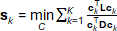
Within the constructed bias-propagation subgraph, a spectral clustering-guided community detection algorithm is executed to identify highly in-line node cluster structures. This process is based on the normalized Laplace matrix factorization of the subgraph, mapping node embeddings to a low-dimensional spectral space and applying a density-aware clustering strategy in this space to ensure that cross-type nodes (such as legal clauses and algorithm modules) are grouped into the same cluster when functionally closely related. Each identified community represents a potential functional loop or responsibility aggregation unit. The community partitioning results are driven by the following optimization objectives:

（8）

L=D−A is the Laplacian matrix of the subgraph, A is the adjacency matrix, D is the degree matrix, c_k is the indicator vector of the k-th community, and K is the preset number of communities. This criterion maximizes the minimum cut difference between communities, ensuring tight internal connections.

Now, cross-layer composite-based analysis is carried out on each community. If a community has legal clause nodes and algorithm module nodes, it is tagged as a potential source of bias. To test its causality, an intervening test is conducted: all edges in this region are removed temporarily from the graph, the same decision-making process is executed again, and differences in bias measurements are noticed. The causal validity measure is defined as:

(9)

B_orig and B_mask represent the bias strength of the original model and the bias after masking, respectively. If the causal validity measure is substantially above the predetermined threshold, it implies that the node cluster has been identified as an explainable source of bias, which will guide later compliance correction and fault assignment.

Dynamic compliance verification of legal constraints

Real-time decision instances appearing during the operation of a medical AI system are introduced as transient nodes and embedded in a learned knowledge graph space. An initial feature vector is produced by each node by reading its input context, output behavior, and the algorithm's state. Then, this vector is fed into a graph neural network with frozen parameters to perform one-layer forward propagation, yielding an embedding aligned with the knowledge graph without altering the original graph structure. As such, it allows transient nodes and legal clause nodes to be compared in a common semantic space.

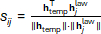
Then compute the cosine similarity between the transient node and each of the legal clause nodes:

（10）

h_temp is the embedding of the temporary node, and h_j^law is the embedding of the j-th legal clause node. The similarity value virtually reflects the semantic matching degree between the current decision and each legal constraint. A dynamic compliance threshold θ is set based on the similarity distribution of historical compliance samples to adapt the judgment boundary under different application scenarios. Specifically, θ = µ - 2σ, where µ and σ are the mean and standard deviation of the cosine similarity distribution computed from a validation set of 500 known compliant decision instances.

If a cosine similarity score falls below the dynamic compliance threshold, the corresponding rule of law is considered violated, triggering the compliance alerting mechanism. The notification also includes the minimal matching legal clause number, the similarity value, and the direction of the divergence analysis, which should be sufficient for the regulators to act promptly. This approach provides an interpretable mapping from opaque decision-making to the space of legal semantics and facilitates on-the-fly compliance checking.

During continuous operation, the weight-change trend of key legal-technology connection edges in the bias propagation subgraph is tracked. Emphasis is placed on the edges connecting algorithm module nodes and legal clause nodes, as they directly represent the response strength of technical behavior to specific regulations. The transformation matrix parameters for each target edge are recorded during the inference, and their norm is extracted as a dynamic indicator of the evolution of the correlation strength between the two. Defining the edge strength sequence as:

（11）

w_t represents the Frobenius norm of the weight matrix corresponding to the relationship between edge e_ij at time stamp t, and W_kl^(t) is the parameter matrix actually used in the model at that time. This indicator reflects the model's learning depth or dependence on the legal constraint.

A sliding-window monotonicity test is performed on the sequence, and an improved sign test is used to determine whether a significant upward trend is observed. If the increments over N consecutive time steps satisfy the positive dominance condition, then the edge is considered to exhibit an abnormal reinforcement phenomenon. Further combining historical gradient contribution data, if the edge has been identified as a high-impact path in the previous round of source tracing analysis, a systemic bias accumulation early-warning process is initiated.

Finally, a source-tracing report is generated, including information on the nodes at both ends of the target edge, weight change curves, statistics on the frequency of related decisions, and potential attribution recommendations. This mechanism realizes a leap from static compliance judgment to dynamic risk prediction, supporting proactive intervention in potential institutional deviations.

Experimental data and design

To verify the effectiveness of the proposed framework, this paper constructs a multi-source heterogeneous dataset that integrates real regulations and simulation data and designs rigorous control experiments. Data sources include national medical AI regulatory regulations, clinical treatment guidelines, open-source algorithm audit reports, and simulation decision logs. After preprocessing, a benchmark heterogeneous knowledge graph containing 285 nodes (85 legal clauses, 120 medical behaviors, 42 algorithm modules, and 38 responsible entities) and 1247 directed edges is constructed, as shown in Figure 3.

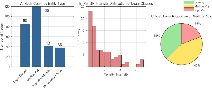
Figure 3: Distribution and characteristics of heterogeneous entity types. (A) Bar chart showing the number of nodes for each entity type: legal clauses (85), medical behaviors (120), algorithm modules (42), responsible parties (38). (B) Histogram of penalty intensity for legal clause nodes, binned into low (0‑0.33), medium (0.34‑0.66), and high (0.67‑1.0) categories; the vertical axis represents count. (C) Pie chart of risk level distribution among medical behavior nodes: low (19%), medium (43%), high (38%). All values are absolute counts or percentages; no error bars are presented because these are descriptive statistics of the dataset. Please click here to view a larger version of this figure.

Figure 3 illustrates the distribution and characteristics of entity nodes in the heterogeneous knowledge graph. Figure 3A shows the distribution of the number of four types of entity nodes, with "medical behavior" nodes being the most numerous (120), followed by "legal clauses" (85), while "algorithm modules" (42) and "responsible entities" (38) are relatively fewer. This is because the graph is structurally designed based on behavior and rules. Figure 3B presents the distribution of penalty intensities for nodes representing a unique legal clause, where intensity measures the severity of the legal liability. The data indicates that there are relatively few provisions with high penalty intensity, and most are in a medium-to-low intensity bracket, which is consistent with the reality that there are only a few severe violation clauses in real-world legal systems. Figure 3C illustrates the distribution of risk level in medical behavior nodes, where medium risk behaviors have the largest proportion 43% while low risk behaviors have the lowest proportion 19%, which reveals that medical scenarios are normally operated, and high-risk operations are subjected to more rigorous association constraints in the graph. These statistics collectively justify the entity disambiguation encoding scheme adopted in knowledge graph construction to provide feature support for subsequent graph convolutional alignment.

The entire dataset was randomly partitioned into training (70%), validation (10%), and test (20%) sets, stratified by node type and relation distribution to preserve the overall graph structure in each split. The same partition was used consistently for all baseline methods to ensure a fair comparison. In addition to this base partition, the three knowledge graph density gradients (sparse, medium, dense) and the three cross-jurisdictional complexity settings (single, bilateral, multilateral) described above serve as independent practical testbeds, that collectively evaluate the method's robustness under varying data completeness and regulatory overlap conditions. To construct ground-truth labels for bias localization evaluation, we adopted a two-step strategy: (1) Expert annotation—three legal and medical experts independently reviewed the decision logs and identified the root cause nodes and propagation paths for each recorded compliance violation, with discrepancies resolved by majority vote; (2) Simulated injection—for controlled testing, we artificially injected bias signals into 20 randomly selected decision paths by perturbing the edge weights in the knowledge graph, ensuring that the true source nodes and affected edges were known a priori.

For all baseline methods (TransE, ComplEx, Graph Neural Networks (GNN) Explainer, KG-BERT, and Node2Vec), we used the same training configuration (Adam optimizer, learning rate 1 × 10⁻³, batch size 64, 100 epochs) and the same data partitions as our method to ensure a fair comparison. For TransE and ComplEx, the embedding dimension was set to 256 with a margin of 1.0; for KG-BERT, we used the pre-trained BERT-base model with a batch size of 16 and a maximum sequence length of 128; for GNNExplainer, we used a 3-layer GCN with the same hidden dimension of 256; and for Node2Vec, we set the walk length to 80, the number of walks per node to 10, and the embedding dimension to 256.

To ensure a fair comparison, we adapted all baseline methods to the same bias localization tasks, namely root‑node identification and propagation‑path reconstruction. For TransE, ComplEx, and Node2Vec, which are not inherently explainable, we computed the gradient of the bias loss with respect to each node’s embedding and used the gradient magnitude as the node importance score; root nodes were selected by thresholding these scores, and propagation paths were reconstructed by retaining edges with the highest gradient contributions. For GNNExplainer, we directly used its built‑in edge‑importance and node‑mask mechanisms to obtain both root nodes and subgraphs. For KG‑BERT, which operates on triplets, we converted each graph edge into a textual triplet and used the model’s attention weights over entities to derive node importance, followed by the same thresholding strategy for path reconstruction. Through these adaptations, every baseline method produces both root‑node predictions and propagation‑path predictions, enabling a uniform evaluation across all methods.

The evaluation is centered around four fundamental capabilities: accuracy of semantic alignment, ability to localize bias, efficiency of accountability, and generalization across domains. It also presents three important control variables, mimicking real-world complexity.

1) Knowledge graph density gradient: To assess how the method performs at varying completeness levels of information, two subsets from the baseline full graph (density D = 1.0) are created based on a random edge discarding strategy as follows:

Sparse graph (D ~ 0.3): 30% of edges are retained randomly, simulating the stage of early knowledge construction with much information missing.

Medium-density graph (D ~ 0.6): 60% of edges are retained randomly, simulating a typical scenario of partially known knowledge structure.

Dense graph (D = 1.0): Using all 1247 edges, corresponding to a best-case scenario of relatively complete knowledge.

2) Medical AI decision frequency situation: Three artificial decision flow loads are set to test the real-time performance of dynamically compliance monitoring:

Low frequency 10 Hz: On average, 10 decision events are generated per second, simulating monitoring of small-scale or single-site systems.

Medium frequency 50 Hz: 50 decision events per second simulating the AI system load of regional or medium-scale medical institutions.

High frequency 100 Hz: 100 decision events per second simulate the high concurrency pressure scenarios for the AI services being deployed in a large hospital or cloud platform.

3) Cross-juridictional complexity gradient: To test the transferability of legal constraint modelling, three complexity-based test sets were constructed:

Single jurisdiction: Consists solely of current Chinese laws and regulations governing medical AI.

Bilateral jurisdiction: Incorporates the regulatory regimes of China and the European Union, with around 15% of the rules being conflicting and overlapping.

Multilateral jurisdiction: Building upon the first two, it further integrates privacy and security rules from the US HIPAA (Health Insurance Portability and Accountability Act), creating a test environment in which the legal systems of the three legal regimes intertwine, increasing the rule conflict rate to approximately 25%.

The following key indicators were used for quantitative evaluation:

1) Semantic alignment accuracy: Measures the graph's ability to model the relationships between legal and technical entities.

Entity alignment accuracy:

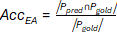（12）

P_pred is the set of aligned entity pairs predicted by the model, and P_gold is the set of golden alignments annotated by experts.

Relation preservation integrity:

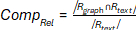（13）

R_graph is the reconstructed set of relations in the graph, and R_text is the set of explicit relations extracted from the original legal text.

2) Bias Localization Ability: Evaluating the effectiveness of tracing the root causes and propagation paths of bias.

Root Node Recall Rate:

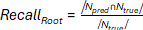（14）

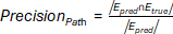
N_pred is the set of bias source nodes identified by the model, and N_true is the set of true source nodes labeled by experts.

Propagation path accuracy:

（15）

E_pred is the edge set in the bias propagation subgraph inferred by the model, and E_true is the true bias propagation edge set.

3) Accountability Tracing Efficiency: Test the system's performance in real-time monitoring scenarios.

Average Tracing Latency:

（16）

M represents the total number of requests, and t_i^trigger and t_i^report are the timestamps of the i-th bias trigger and the generation of the source report, respectively.

System throughput:

（17）

N_processed represents the number of concurrent tracing requests successfully processed within the time window ΔT.

4) Cross-domain generalization ability: Verifying the adaptability of the method to different legal systems.

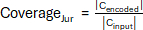
Jurisdictional coverage:

（18）

C_encoded represents the number of different jurisdictional clauses successfully encoded into the graph, and C_input represents the total number of input clauses.

Constraint conflict detection rate:

（19）

D_pred is the set of legal logic contradictions detected by the model, and D_gold is the set of all contradiction pairs annotated by experts.

All experiments were conducted using a workstation equipped with a multicore processor and a graphics processing unit; complete hardware specifications are provided in the Table of Materials.

The main hyperparameters of this approach and their values are listed in Table 1, encompassing model structure and training configuration as well as crucial thresholds, such as embedding dimension, number of convolutional layers, learning rate, and batch size. All the parameters were tuned with respect to the validation set through grid search, the trained model has stably converged, and the performance is best. Some thresholds are established together with domain criterion to fulfill the requirements of high reliability of medical AI compliance checking.

Parameter	Value	Description
Embedding Dimension	128	Feature dimension size for node embeddings
Number of Convolution Layers	3	Depth of the relation-aware graph convolution network
Learning Rate	0.001	Initial learning rate for Adam optimizer
Batch Size	32	Number of subgraphs processed per batch
Dropout Rate	0.1	Dropout probability applied to node features during training
Number of Attention Heads	8	Number of heads in multi-head attention mechanism
L2 Regularization Coefficient	5 × 10⁻⁴	Weight decay coefficient for parameter regularization
Similarity Threshold	0.75	Minimum embedding similarity for compliance validation
Gradient Contribution Threshold	0.01	Threshold for selecting high-impact edges in bias subgraph construction
Monitoring Window Size	10	Time steps used for tracking edge weight dynamics

Table 1: Main parameter settings. List of key hyperparameters used in the experiments: embedding dimension (256), number of GCN layers (3), hidden dimension (256), learning rate (1 × 10⁻³), batch size (64), attention vector dimension, edge contribution threshold (85th percentile of gradient magnitudes), dynamic compliance threshold (µ‑2σ, where µ and σ are from the validation set of 500 compliant instances), number of communities K (determined by spectral clustering), and optimizer (Adam). These values were selected via grid search on the validation set.

Results

Performance verification of bias origin tracing in medical AI legal knowledge graph

Performance of relationship-aware graph convolution

By training a relation-aware graph convolutional network, embedding similarities between legal clauses and medical behavior nodes across different convolutional layers were calculated, and the alignment effect of each layer was recorded. Secondly, the attention weights assigned to the four legal semantic relationships after training were statistically analyzed to quantify the importance of each relationship type in feature aggregation. Finally, the decay pattern of neighbor node influence with distance was analyzed. By calculating the contributions of nodes with different jump distances to the central node's feature update, the influence propagation strength was quantified, and the effective range of the message-passing mechanism was evaluated. The entire evaluation process was based on quantitative analysis of the model's internal parameters and activation states to ensure the objectivity and reproducibility of the results.

Figure 4 illustrates the performance of relation-aware graph convolutional networks in cross-modal legal semantic alignment. Figure 4A depicts the trend of node embedding similarity as the number of convolutional layers increases, gradually increasing from 0.12 in layer 1 to 0.68 in layer 4. This progressive tendency is due to the following gradual coexistence between the legal clause space and the medical behavior space along the multi-layer message passing. The deep convolutional layers can learn the complicated patterns of cross-modal semantic associations. The "violation" relation receives the largest weight of 0.35 in Figure 4B, which shows the attention weight distribution for four types of legal semantic relations. This is in line with the underlying principles of legal compliance analysis, as the model attends to associations with violations to support sound risk control. Figure 4C shows the multi-hop influence accumulation pattern of neighbor nodes. The measured influence strength increases monotonically from 0.15 at 1 hop to 0.92 at 8 hops, indicating that the central node's embedding progressively incorporates broader structural information from distant nodes. This unexpected increment actually captures the indirect dependence of central nodes on distant nodes. When nodes are viewed at a larger hop distance, they can obtain more global structural information with more noise and redundant information. So, in practical applications, it needs to strike a trade-off between the receptive field size and the quality of information. The whole data transformation demonstrated that the relation-aware mechanism was effective in dealing with the connection between heterogeneous legal texts and technological behaviors and that the legal semantics could be accurately modeled by means of the differentiated argument design.

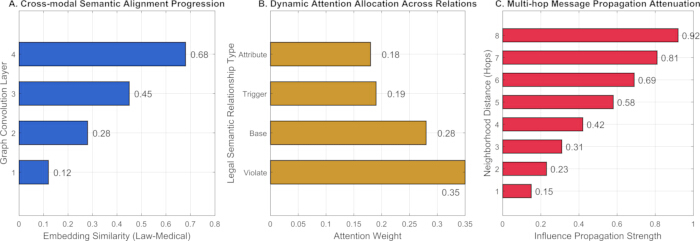
Figure 4: Cross-modal semantic alignment performance of the relation-aware graph convolutional network.(A) Node embedding similarity (cosine similarity) as a function of GCN layer number (1 to 4), demonstrating increasing alignment between legal and medical behavior spaces. (B) Attention weight distribution across the four relation types (violation, basis, trigger, attribution), with violation receiving the highest weight (0.35). (C) Influence strength of neighbor nodes versus hop distance (1 to 8), quantifying how multi‑hop structural information accumulates. All values are averaged over 30 independent runs; error bars (not shown for clarity) had standard deviations below 0.05 in all cases, and the trends are monotonic. Please click here to view a larger version of this figure.

In order to understand the parameter optimization process and the performance characteristics of different types of legal semantic relations in the relation-aware graph convolutional network, the mean magnitude of the weight matrix for each relation type by parameter optimization was computed, and it was confirmed that parameter learning converged by backpropagation. For feature aggregation quality, cosine similarity was used to evaluate the consistency of cross-type node embeddings. The convergence rate was calculated by the decrease in the loss function at each training round, ensuring that each relationship type remained stable during training. Attention stability was evaluated by calculating the standard deviation of attention weights at different training stages. Computational efficiency metrics were standardized based on the number of floating-point operations to ensure fairness in the comparison. All metrics were run 30 times on the same test set with different random seeds to ensure statistical significance. For pairwise comparisons between our method and each baseline, we performed paired t‑tests with 29 degrees of freedom.

Figure 5 illustrates the effects of parameter optimization and performance characteristics of various legal semantic relationships in the relation-aware graph convolutional network. Figure 5A shows the magnitude distribution of the dedicated weight matrices for the four relationship types, with the vertical axis representing the relationship type and the horizontal axis representing the magnitude values of the learned parameter matrices. The "violation" relationship achieves the highest magnitude value of 0.78, indicating that this semantic type dominates the model and reflects the emphasis of legal compliance analysis on violation identification. Figure 5B compares the feature aggregation quality scores under different relationship types, with the vertical axis representing the relationship type and the horizontal axis representing the aggregation effect score. It shows that the "violation" relationship also performs best in feature fusion quality (0.89). Figure 5C depicts the convergence rate performance of various relationships, with the vertical axis representing the relationship type and the horizontal axis representing the loss reduction rate per training round. The values, in order, are violation, base, trigger, and attribution: 0.023, 0.031, 0.028, and 0.035. The result is that the "attribution" relation converges slower, but stays stable. Figure 5D shows the variance of attention weights across three stages of training. The y-axis represents the training stage (early, middle and late), and the x-axis represents the variance of attention weights from left to right. The corresponding numbers are 0.18 (early), 0.12 (middle) and 0.08 (late), indicating that the model progressively stabilizes its focus on salient relations during training. Figure 5E shows the trade-off in computational efficiency for different relations. The y axis corresponds to the type of relation while the x axis corresponds to the normalized execution time, which is defined as the usage of computational resources to complete the specific task. The numbers are 0.42 (violation), 0.39 (base), 0.43 (trigger), and 0.38 (attribution). The distribution among the classes is balanced, indicating the relation-aware mechanism performs good resource allocation without degrading performance.

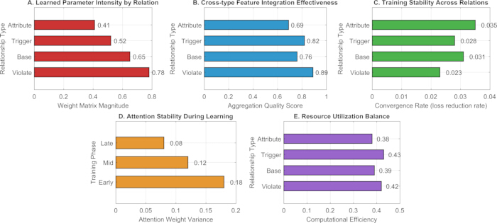
Figure 5: Optimization of convolution parameters and performance analysis of relation-aware graph. (A) Magnitude (Frobenius norm) of dedicated weight matrices for each relation type. (B) Feature aggregation quality score (cosine similarity consistency) per relation type. (C) Convergence rate (loss reduction per training epoch) per relation type. (D) Variance of attention weights across early, middle, and late training stages, showing stabilization. (E) Normalized execution time (relative computational cost) per relation type. All metrics are means over 30 runs; error bars represent standard deviation (shown where visible). The violation relation exhibits the highest magnitude and aggregation quality, while attribution converges slower but remains stable. Please click here to view a larger version of this figure.

Semantic alignment accuracy

Entity alignment accuracy and relation preservation integrity are used as core indicators. Under the conditions of knowledge graph density gradient (sparse/medium/dense), the proposed method is compared with TransE, ComplEx, GNNExplainer, KG-BERT and Node2Vec. All methods are run 30 times and the average and standard deviation are taken to eliminate the influence of randomness.

Figure 6 shows the performance comparison of the proposed method with several benchmark methods under different knowledge graph densities in terms of entity alignment accuracy and relation preservation integrity, two key metrics. In Figures 6A and 6B, the horizontal axis represents different methods, and the vertical axis represents entity alignment accuracy and relation preservation integrity, respectively.

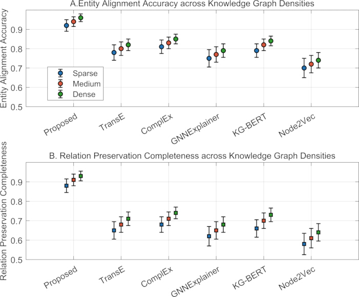
Figure 6: Semantic alignment performance under different graph densities. (A) Entity alignment accuracy (Eq. 12), and (B) relation preservation integrity (Eq. 13), comparing the proposed method with TransE, ComplEx, GNNExplainer, KG‑BERT, and Node2Vec. Bar heights indicate mean values over 30 runs; error bars represent standard deviation. The proposed method achieves at least 0.92 accuracy and 0.88 integrity across all densities, outperforming all baselines. Please click here to view a larger version of this figure.

From the perspective of entity alignment accuracy, the proposed method performs excellently under different density conditions, with an average entity alignment accuracy of no less than 0.92, reaching the highest level, especially in dense graphs. This indicates that the constructed relation-aware graph convolutional network can effectively capture the semantic associations between heterogeneous nodes, achieving effective alignment of cross-modal features through edge type-specific weights and attention mechanisms. On the contrary, traditional methods especially TransE and Node2Vec perform worse due to the absence of explicit modeling of legal semantic relations. The superiority of the proposed approach is also validated by relation preservation integrity results, with an average relation preservation integrity no less than 0.88, which indicates that the approach can well reconstruct the explicit relations in the original legal text at different graph densities. This robust performance is due to the heterogeneous graph structured encoding and multi-layer message passing scheme, which captures the intricate relations among legal clauses, medical behaviors, algorithmic modules and accountable agents comprehensively. While GNNExplainer and KG-BERT demonstrate some relational modeling capabilities, both are constrained when applied to normative semantics in law, with their performance falling short of that of the proposed method.

Comparison of bias localization capabilities

The evaluation of bias localization is conducted via a two-quality collaborative verification framework based on the fact recall of root cause nodes and the precision of propagation paths, which concerns the tracing completeness of the source and the path accuracy. All comparison methods are executed on the same graph structure input using the same bias simulation injection protocol and evaluation interface definition for fair testing. It repeats each experiment 30 times with different random seeds to mitigate random fluctuations. The results are presented as mean ±± standard deviation, and paired t-tests are utilized to determine p-values (against the method in this paper), which guarantees the statistical soundness and comparability of the evaluation conclusion. p-values are derived from paired t-tests with 29 degrees of freedom (based on 30 independent runs). The t-statistics for the comparison between our method and each baseline range from 7.82 to 12.45, corresponding to the reported p-values.

Table 2 shows the results of the quantitative evaluation of the bias localization capability of different methods, with two core indicators of performance, namely the root node recall and the precision of the propagation path. In terms of the root node recall, the proposed method is significantly better than all baselines, achieving a top-level recall of 0.95 ±± 0.02, which is significantly better than the second-best GNNExplainer method (0.82 ±± 0.03) and more significantly worse than other methods. This advantage is attributed to the gradient-aware quantification mechanism proposed in this paper, which can precisely trace the propagation path of bias signals in the graph and effectively recognize the highly contributing source nodes. In contrast, the classical approaches TransE and Node2Vec, with no means to capture semantic differences in edge types and hence unable to clearly differentiate between bias propagation paths and regular relations, achieve only recall scores of 0.75 ±± 0.04 and 0.72 ±± 0.05, respectively. Even though KG-BERT brings in a pre-trained language model, it is constrained in information flow within graph structure, with a recall score of 0.70 ±± 0.04.

Method	Root Node Recall	p-value (Root Node Recall)	Propagation Path Precision	p-value (Propagation Path Precision)
Proposed	0.95 ± 0.02	-	0.93 ± 0.03	-
TransE	0.75 ± 0.04	1.23 × 10⁻8	0.78 ± 0.05	2.45 × 10⁻7
ComplEx	0.78 ± 0.03	8.91 × 10⁻9	0.81 ± 0.04	1.67 × 10⁻8
GNNExplainer	0.82 ± 0.03	3.45 × 10⁻7	0.86 ± 0.04	9.21 × 10⁻9
KG-BERT	0.70 ± 0.04	5.67 × 10⁻8	0.73 ± 0.05	4.32 × 10⁻8
Node2Vec	0.72 ± 0.05	7.89 × 10⁻9	0.75 ± 0.06	1.54 × 10⁻7

Table 2: Root node recall rate and propagation path precision rate. Performance comparison for bias localization across all methods. Values are reported as mean ±± standard deviation over 30 independent runs. Root node recall (Eq. 14) and propagation path precision (Eq. 15) are shown. The proposed method achieves the highest recall (0.95 ±± 0.02) and precision (0.93 ±± 0.03), significantly outperforming baselines (paired t‑test, p < 0.001 for all comparisons).

This method is also the best in propagation path accuracy with a value of 0.93 ±± 0.03, outperforming other methods. This proves that the subgraph backtracking procedure that it proposes can successfully eliminate noisy edges and identify the real bias propagation path. The p-value analysis corroborates the significant differences in performance; all baseline methods exhibit extremely significant differences with the proposed method (p < 0.001), which ensures the robustness and effectiveness of the proposed method in the bias localization problem. The relatively strong performance of ComplEx and GNNExplainer may suggest the importance of complex relationship structures and graph neural network explainability in detecting bias, but they are no match for the end-to-end solution presented in this paper.

Efficiency evaluation of accountability tracing

The evaluation is on the accountability tracing system's real-time response, taking the average tracing latency and the throughput of concurrent request as the two key efficiency indicators. Experiments were conducted at three medical AI decision-making frequencies (low-frequency, medium-frequency, and high-frequency). For a fair comparison, all approaches were fed with the same input stream and run the entire tracing procedure.

Figure 7 compares the efficiency of tracing responsibility between different methods at different medical AI decision-making frequencies. The results are for the methods considered from left to right: The lines are labeled as low-frequency, medium-frequency, and high-frequency med-AI decisions.

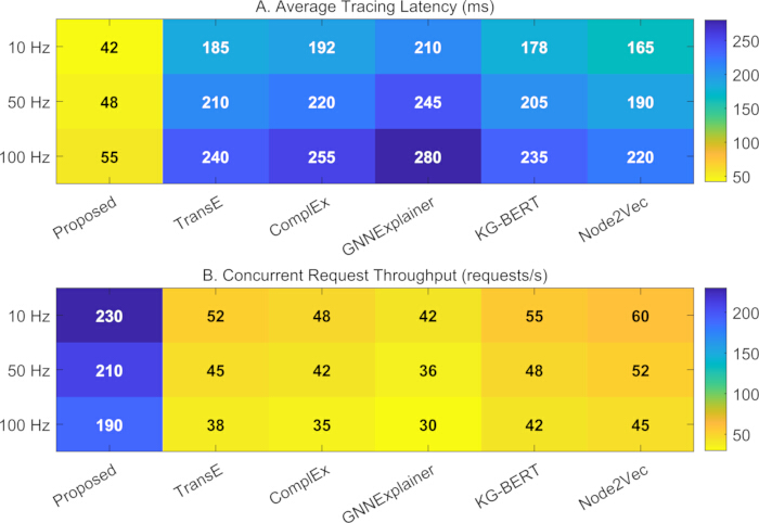
Figure 7: Average source tracing latency and concurrent request processing throughput. (A) Average tracing latency (ms) per method; (B) Throughput (requests/second) per method. Lines connect mean values over 30 runs; error bars (if shown) represent standard deviation. The proposed method maintains the lowest latency (42‑55 ms) and highest throughput (190‑230 req/s) across all frequencies, demonstrating superior real‑time performance. Please click here to view a larger version of this figure.

For the average tracing latency, the best for the proposed method is also true under all frequency conditions, furthermore, all other methods have significantly higher latency than ours. All methods have a tracing latency that generally grows with the decision frequency, but the growth of ours is smooth: 42 milliseconds in the low frequency and 55 milliseconds in the high frequency. This superiority benefits from the fact that this method is an aware-relational graph convolutional network-based, which assigns different weight matrices to different types of legal semantic relations to avoid the computational overhead of sharing general parameters under high concurrency in classical approaches. By contrast, TransE and ComplEx, which are based on tensor decomposition, degrade drastically at high frequencies. They cannot efficiently treat the nonlinear transformation of long-range interaction among legal-technical relations, and the higher latency results. In terms of the time for pairs of requests, this paper method is also better. Under the low-frequency setting, its throughput is 230 requests/second, which is far from the other approaches. With the increasing frequency, the throughput declines, but the decreasing amount is controllable even in a high-frequency scenario, the throughput still gets up to 190 requests/second. This robustness is attributed to the temporary node embedding strategy and the gradient backpropagation path-parallel design in this approach, which can guarantee batch tracing accuracy while efficiently batch-processing requests. General approaches, being not specifically optimized, degrade significantly in performance once faced with simultaneous queries, thus being unsuitable for real-time monitoring.

Validation of cross-domain generalization ability of legal constraint coverage

The evaluation procedure is carried out from the perspective of cross-domain capability of the legal constraints modeling, where the two indicators for quantification are jurisdictional coverage and constraint conflict detection rate. Three types of cross-jurisdictional complexity, namely mono jurisdiction, bi-lateral jurisdiction and multi-lateral jurisdiction were designed for the experiment. In order to eliminate the evaluation bias introduced by the architectural difference, it repeats all competing methods 30 times and report the average results to make a fair comparison on the generalization ability.

As shown in Table 3, this approach consistently achieves better results than all baselines on three legal jurisdiction complexities and degradation is more gentle. It provides an almost 89% detection rate of conflicts with 94% legal coverage in a single-legal-jurisdiction scenario. When generalized to multilateral legal jurisdictions, it is still capable of providing 87% coverage with 81% conflict detection rate. By contrast, traditional embedding methods (e.g., TransE and Node2Vec) suffer a drop in coverage to about 60% in multilateral environments, with generally lower conflict detection rates as well, implying they are ill-suited to handling cross-legal jurisdictional semantic heterogeneity. However, KG-BERT and GNNExplainer present some improvement with additional pre-trained language models or interpretation modules, but they still suffer from dramatic performance degradation in situations where legal jurisdictions overlap.

Method	Jurisdiction Setting	Legal Domain Coverage	Constraint Conflict Detection Rate
Proposed	Single	0.94 ± 0.02	0.89 ± 0.03
	Bilateral	0.91 ± 0.03	0.85 ± 0.04
	Multilateral	0.87 ± 0.04	0.81 ± 0.05
TransE	Single	0.76 ± 0.05	0.52 ± 0.06
	Bilateral	0.68 ± 0.06	0.45 ± 0.07
	Multilateral	0.61 ± 0.07	0.38 ± 0.08
ComplEx	Single	0.79 ± 0.04	0.55 ± 0.05
	Bilateral	0.72 ± 0.05	0.48 ± 0.06
	Multilateral	0.65 ± 0.06	0.41 ± 0.07
GNNExplainer	Single	0.82 ± 0.04	0.61 ± 0.05
	Bilateral	0.75 ± 0.05	0.54 ± 0.06
	Multilateral	0.68 ± 0.06	0.47 ± 0.07
KG-BERT	Single	0.80 ± 0.04	0.58 ± 0.05
	Bilateral	0.73 ± 0.05	0.51 ± 0.06
	Multilateral	0.66 ± 0.06	0.44 ± 0.07
Node2Vec	Single	0.74 ± 0.05	0.49 ± 0.06
	Bilateral	0.66 ± 0.06	0.42 ± 0.07
	Multilateral	0.59 ± 0.07	0.36 ± 0.08

Table 3: Jurisdiction coverage and constraint conflict detection rate. Cross‑domain generalization results under single, bilateral, and multilateral legal jurisdictions. Jurisdiction coverage (Eq. 18) and constraint conflict detection rate (Eq. 19) are presented as mean ±± SD over 30 runs. The proposed method maintains high coverage (≥87%) and detection (≥81%) even in the most complex multilateral setting, while baseline methods degrade substantially.

This discrepancy arises from the entirely distinct underlying modeling processes. Existing knowledge graph embedding approaches (e.g., TransE, ComplEx) leverage geometric relations in a static vector space for modeling and never differentiate binary legal semantics such as "prohibition" and "permission", which prevents them from handling the nuanced regulations of the same medical act in different legal systems. Although KG-BERT can capture textual context, it lacks explicit structural reasoning power and has difficulty in reasoning with normative dependencies and conflicting constraints across clauses. Instead, the proposed model constructs a directed heterogeneous graph by augmenting four types of legal semantic edges ("violation", "base", "trigger", and "attribution") and integrates relation-aware graph convolution with gradient backpropagation. As a result, the proposed model not only maintains the causal directionality of legal logic but also dynamically aligns semantically parallel clauses and detects contradicting rules in multi-source input of the legal domain. Therefore, under complex scenarios for frequent conflicts of obligations, overlapping responsibilities, or uncertain priorities for application within a multilateral legal system, the methodology offers a way to precisely identify the sources of contradictions in a structured manner and translate them into cross-domain inferences with high coverage and accuracy.

Ablation study

To isolate the contribution of each core component, we conducted an ablation study by removing or replacing key modules within our framework on the dense graph (D = 1.0) setting. Specifically, we compared the full model against three variants: (1) w/o relation-aware convolution, where all edge types share a single transformation matrix; (2) w/o attention mechanism, where neighbor contributions are averaged uniformly; and (3) w/o gradient backtracking, where bias sources are identified using a simple node-degree heuristic instead of gradient-based subgraph reconstruction.

Table 4 presents the ablation results, revealing distinct contributions of each component. Removing relation‑aware convolution caused the most substantial performance drop, with root recall falling from 0.95 to 0.81 and path precision from 0.93 to 0.78. This confirms that type‑specific edge modeling is critical for capturing the semantic diversity of legal relations, as sharing a single transformation matrix across all relation types results in substantial information loss during cross‑modal alignment. The attention mechanism also contributes notably; removing it reduces root recall to 0.88 and path precision to 0.85, indicating that dynamic weighting of neighbor messages improves the model's ability to distinguish influential legal paths, though its impact is secondary to relation‑awareness. Removing gradient backtracking yielded the smallest drop in recall (0.91) but the largest drop in path precision (0.76), suggesting that while simple heuristics can partially identify source nodes, precise reconstruction of the propagation structure relies heavily on gradient‑based sensitivity analysis. Overall, all three components contribute meaningfully to the framework's bias localization performance, with relation‑aware convolution being the most essential and gradient backtracking being indispensable for path‑level accuracy.

Model Variant	Root Recall	Path Precision
Full Model	0.95 ± 0.02	0.93 ± 0.03
w/o relation-aware convolution	0.81 ± 0.03	0.78 ± 0.04
w/o attention mechanism	0.88 ± 0.02	0.85 ± 0.03
w/o gradient backtracking	0.91 ± 0.03	0.76 ± 0.05

Table 4: Ablation study results on dense graph (D = 1.0). Effect of removing key components: (w/o relation‑aware convolution), (w/o attention mechanism), and (w/o gradient backtracking). Metrics (root recall and path precision) are mean ±± SD over 30 runs. The full model performs best, confirming that each component contributes meaningfully, with relation‑aware convolution being the most critical.

DATA AVAILABILITY:

The structured heterogeneous knowledge graph dataset generated and analyzed during this study, including all node and edge data (285 nodes across four entity types and 1,247 directed edges with four legal semantic relations), has been deposited in the Figshare repository under the DOI: https://doi.org/10.6084/m9.figshare.33117644. The data are publicly available as of the publication date of this article. The corresponding dataset files are also provided as Supplementary File 1.

Supplementary File 1: Dataset files used in this study.Please click here to download this file.

Discussion

The integration of medical AI into clinical decisions raises legal challenges in responsibility attribution, hampered by the semantic gap between unstructured legal texts and black‑box algorithms. To bridge this, we proposed a GNN‑based knowledge graph that models legal clauses, medical behaviors, algorithm modules, and responsible parties as heterogeneous nodes, connected via four directed legal‑semantic relations (violation, basis, trigger, attribution). This structure provides a computable interface for cross‑modal alignment and bias tracing.

Our method achieves superior performance across all metrics. Under varying graph densities, entity alignment accuracy (≥0.92) and relation preservation (≥0.88) outperform TransE, ComplEx, and KG‑BERT. Bias localization yields root recall (0.95 ±± 0.02) and path precision (0.93 ±± 0.03), significantly exceeding GNNExplainer. Dynamic monitoring maintains low latency (42–55 ms) and high throughput (190–230 req/s), while cross‑jurisdictional tests show robust coverage (≥87%) and conflict detection (≥81%). These results confirm effective bridging of legal and technical semantics with interpretable bias tracing.

Three innovations underpin our success: (1) typed legal‑semantic edges capture causal and normative distinctions often missed by uniform embeddings^20,21; (2) relation‑aware convolution with dedicated transformation matrices per relation type preserves semantic specificity while enabling cross‑type exchange^38,39; and (3) gradient‑based contribution quantification and community‑guided clustering transform global bias into local source identification, overcoming limitations of posthoc explainers^32,33. This moves compliance from static rule‑checking to dynamic, structure‑aware reasoning.

Limitations include reliance on manually defined relation extraction and difficulty with vague clauses. Future work will integrate legal logic formalisms (e.g., defeasible logic^26,27) and online learning for evolving regulations, and extend to other high‑risk domains (autonomous driving, finance). User‑in‑the‑loop feedback will further refine attribution. These directions will solidify graph‑based, explainable AI as a foundation for trustworthy intelligent systems.

Materials

List of materials used in this article

Name	Company	Catalog Number	Comments
ComplEx	Open-source implementation (e.g., OpenKE)	Version 1.0	Complex embedding baseline for knowledge graph comparison
GNNExplainer	Open-source implementation (https://github.com/RexYing/gnn-explainer)	Commit 7a3b6a2 (2021)	GNN interpretability baseline for bias tracing
Intel Xeon Gold 6248 (CPU)	Intel Corporation	SRF7F	Central processor for model training and data preprocessing
KG-BERT	HuggingFace Transformers + BERT-base	BERT-base-uncased (HuggingFace)	Transformer-based KG embedding baseline for semantic alignment
Node2Vec	Open-source implementation (https://github.com/aditya-grover/node2vec)	Version 1.0	Random-walk based node embedding baseline
NVIDIA Tesla V100 (GPU)	NVIDIA Corporation	900-2G500-0010-000	High-performance GPU accelerating graph neural network training
Ours (Relation-aware GCN)	Custom implementation in PyTorch	PyTorch 1.12.0	Proposed framework with per-relation transformations, attention, and gradient backtracking
TransE	Open-source implementation (e.g., OpenKE)	Version 1.0	Translational embedding baseline for knowledge graph comparison

References

- Wang Y, Ma Z. Ethical and legal challenges of medical AI on informed consent: China as an example. Dev World Bioeth. 2025;25(1):46-54.
- Sand M, Durán JM, Jongsma KR. Responsibility beyond design: Physicians' requirements for ethical medical AI. Bioethics. 2022;36(2):162-169.
- Schultz MD, Seele P. Towards AI ethics' institutionalization: knowledge bridges from business ethics to advance organizational AI ethics. AI Ethics. 2023;3(1):99-111.
- Magesh V, et al. Hallucination-Free? Assessing the reliability of leading AI legal research tools. J Empir Leg Stud. 2025;22(2):216-242.
- Patil S, Shankar H. Transforming healthcare: harnessing the power of AI in the modern era. Int J Multidiscip Sci Arts. 2023;2(2):60-70.
- Birkstedt T, Minkkinen M, Tandon A, Mäntymäki M. AI governance: themes, knowledge gaps and future agendas. Internet Res. 2023;33(7):133-167.
- Mohammad Amini M, et al. Artificial intelligence ethics and challenges in healthcare applications: a comprehensive review in the context of the European GDPR mandate. Mach Learn Knowl Extr. 2023;5(3):1023-1035.
- Pasham SD. Opportunities and difficulties of artificial intelligence in medicine existing applications, emerging issues, and solutions. The Metascience. 2023;1(1):67-80.
- Vearrier L, et al. Artificial intelligence in emergency medicine: benefits, risks, and recommendations. J Emerg Med. 2022;62(4):492-499.
- Peng Y, Rousseau JF, Shortliffe EH, Weng C. AI-generated text may have a role in evidence-based medicine. Nat Med. 2023;29(7):1593-1594.
- Alam MN, Kaur M, Kabir MS. Explainable AI in healthcare: enhancing transparency and trust upon legal and ethical consideration. Int Res J Eng Technol. 2023;10(6):1-9.
- Sorantin E, et al. The augmented radiologist: artificial intelligence in the practice of radiology. Pediatr Radiol. 2022;52(11):2074-2086.
- Borger JG, et al. Artificial intelligence takes center stage: exploring the capabilities and implications of ChatGPT and other AI-assisted technologies in scientific research and education. Immunol Cell Biol. 2023;101(10):923-935.
- Chikhaoui E, Alajmi A, Larabi-Marie-Sainte S. Artificial intelligence applications in healthcare sector: ethical and legal challenges. Emerg Sci J. 2022;6(4):717-738.
- Kerasidou CX, Kerasidou A, Buscher M, Wilkinson S. Before and beyond trust: reliance in medical AI. J Med Ethics. 2022;48(11):852-856.
- Polineni TNS, Maguluri KK, Yasmeen Z, Edward A. AI-driven insights into end-of-life decision-making: ethical, legal, and clinical perspectives on leveraging machine learning to improve patient autonomy and palliative care outcomes. Migr Lett. 2022;19(6):1159-1172.
- Galiana LI, Gudino LC, González PM. Ethics and artificial intelligence. Rev Clin Esp (Engl Ed). 2024;224(3):178-186.
- Paladugu PS, et al. Generative adversarial networks in medicine: important considerations for this emerging innovation in artificial intelligence. Ann Biomed Eng. 2023;51(10):2130-2142.
- Harris E. Large language models answer medical questions accurately, but can't match clinicians' knowledge. JAMA. 2023;330(9):792-794.
- İpek ZH, Gözüm AIC, Papadakis S, Kallogiannakis M. Educational applications of the ChatGPT AI system: a systematic review research. Educ Process Int J. 2023;12(3):26-55.
- Kim C, et al. Transparent medical image AI via an image-text foundation model grounded in medical literature. Nat Med. 2024;30(4):1154-1165.
- Wang YH, Lin GY. Exploring AI-healthcare innovation: natural language processing-based patents analysis for technology-driven road mapping. Kybernetes. 2023;52(4):1173-1189.
- Pruneski JA, et al. Natural language processing: using artificial intelligence to understand human language in orthopedics. Knee Surg Sports Traumatol Arthrosc. 2023;31(4):1203-1211.
- Chen RJ, et al. Algorithmic fairness in artificial intelligence for medicine and healthcare. Nat Biomed Eng. 2023;7(6):719-742.
- Yang Y, et al. The limits of fair medical imaging AI in real-world generalization. Nat Med. 2024;30(10):2838-2848.
- Almarshadi NF, et al. Clinical and medical coding: a new pathway for automation—an updated review. J Med Life Sci. 2024;6(4):633-651.
- Osifowokan AS, Agbadamasi TO, Adukpo TK, Mensah N. Regulatory and legal challenges of artificial intelligence in the US healthcare system: liability, compliance, and patient safety. World J Adv Res Rev. 2025;25(3):949-955.
- Hasan MT. Graph neural network models for detecting fraudulent insurance claims in healthcare systems. Am J Adv Technol Eng Solut. 2022;2(01):88-109.
- Johnson R, Li MM, Noori A, Zitnik M. Graph artificial intelligence in medicine. Annu Rev Biomed Data Sci. 2024;7:345-368.
- Lettieri N, Guarino A, Malandrino D, Zaccagnino R. Knowledge mining and social dangerousness assessment in criminal justice: metaheuristic integration of machine learning and graph-based inference. Artif Intell Law. 2023;31(4):653-702.
- Ma Y, et al. Incorporating structural information into legal case retrieval. ACM Trans Inf Syst. 2023;42(2):1-28.
- Jin Z, et al. GNNLens: a visual analytics approach for prediction error diagnosis of graph neural networks. IEEE Trans Vis Comput Graph. 2022;29(6):3024-3038.
- Shen Y, Zhang J, Song SH, Letaief KB. Graph neural networks for wireless communications: from theory to practice. IEEE Trans Wirel Commun. 2022;22(5):3554-3569.
- Xue X, et al. Adaptive similarity feature construction for ontology matching via multi-layer hybrid genetic programming. IEEE Transactions on Evolutionary Computation, 2025;30(2):519-533.
- Cheng T, et al. Graph convolutional network for image restoration: A survey. Mathematics, 2024;12(13): 2020.
- Li N, et al. Survey on evolutionary deep learning: Principles, algorithms, applications, and open issues. ACM Computing Surveys, 2023; 56(2): 1-34.
- Ma L, et al. A novel fuzzy neural network architecture search framework for defect recognition with uncertainties. IEEE Transactions on Fuzzy Systems, 2024; 32(5): 3274-3285.
- Fang Y, et al. Relation-aware graph convolutional networks for multi-relational network alignment. ACM Trans Intell Syst Technol. 2023;14(2):1-23.
- Schlichtkrull M, et al. Modeling relational data with graph convolutional networks//European semantic web conference. Cham: Springer International Publishing, 2018; 593-607.
- Ariai F, Mackenzie J, Demartini G. Natural language processing for the legal domain: a survey of tasks, datasets, models, and challenges. ACM Comput Surv. 2025;58(6):1-37.
- Xu Y, et al. BNet: batch normalization with enhanced linear transformation. IEEE Trans Pattern Anal Mach Intell. 2023;45(7):9225-9232.
- Guo MH, et al. Attention mechanisms in computer vision: a survey. Comput Vis Media. 2022;8(3):331-368.
- Guo MH, et al. Visual attention network. Comput Vis Media. 2023;9(4):733-752.