Mixture-of-Experts Electroencephalography-Functional Magnetic Resonance Imaging Fusion for Interpretable Computer-Assisted Brain Disorder Diagnosis

Summary

This protocol presents Brain Mixture-of-Experts, an adaptive and interpretable Electroencephalography-functional magnetic resonance imaging fusion framework for computer-assisted diagnosis of brain disorders. The method integrates heterogeneous EEG and fMRI representations through modality-specific experts, a shared neural-state expert, and adaptive routing, while maintaining interpretability and inference under simulated missing-modality conditions.

Abstract

Electroencephalography (EEG) and functional magnetic resonance imaging (fMRI) provide complementary information about brain function, and have shown significant promise in detecting functional abnormalities in various brain disorders. However, the distinct signal characteristics and disparate representational spaces of EEG and fMRI pose severe challenges to effective multimodal fusion, thereby hindering accurate computer-assisted diagnosis of brain disorders with conventional fixed models. This study presents Brain Mixture-of-Experts (BrainMoE), an adaptive and interpretable EEG-fMRI fusion framework for computer-assisted diagnosis of brain disorders, integrating multimodal brain features through modality-specific experts, a shared neural-state expert, and an adaptive routing mechanism. BrainMoE first projects EEG and fMRI signals into a unified Desikan-Killiany (DK) atlas region-of-interest (ROI) space, then uses graph encoders to extract modality-specific brain-network representations. The soft-routing module produces a routing representation, and the Expert Gate in the Fuse Module generates sample-specific weights to combine the EEG, fMRI, and shared neural-state expert representations. To handle incomplete acquisition scenarios, modality-state masks and missing-modality tokens are incorporated, allowing the same trained model to perform full EEG-fMRI, EEG-only, and fMRI-only inference. Finally, node-occlusion analysis provides ROI-level attribution maps for both EEG- and fMRI-derived predictions. The framework was evaluated on the Healthy Brain Network (HBN) dataset across five binary brain disorder classification tasks, including major depressive disorder, anxiety disorder, reading impairment, autism spectrum disorder, and attention-deficit/hyperactivity disorder. BrainMoE outperformed state-of-the-art comparison algorithms, achieving an average AUC of 86.9 ± 3.0%, and ablation experiments supported the contribution of the routing and expert-fusion components. Furthermore, the interpretability analysis identifies group-level ROI contributions to disease classification that are consistent with previously reported neuroimaging findings. This method supports computer-assisted diagnosis of brain disorders by addressing the challenge of integrating heterogeneous EEG-fMRI neural representations while maintaining interpretability and inference under simulated missing-modality conditions.

Introduction

Brain disorders involve complex changes in neural activity and brain network organization that are difficult to characterize with a single imaging modality¹. After source reconstruction², EEG provides region-level electrophysiological (EEG) activity, whereas functional magnetic resonance imaging (fMRI) captures region-level functional connectivity, offering complementary views of brain function. To facilitate their integration, prior multimodal work has mapped both modalities to the 68-region Desikan-Killiany (DK) atlas³. Although this spatial correspondence does not imply equivalence in temporal resolution or physiological origin, it provides a unified anatomical index for node-level graph fusion, fixed graph dimensions, and consistent region-of-interest (ROI) level interpretation while preserving modality-specific information. Integrating these anatomically aligned yet modality-specific representations can enrich disease-related brain-signal representations and support computer-assisted brain-disorder diagnosis^3,4.

Despite the potential of EEG-fMRI fusion for computer-assisted diagnosis of brain disorders, the heterogeneity between the two modalities poses a technical challenge to their effective integration. Classical machine learning methods, such as SVM and MLP, can provide baseline classification models, but they have limited capacity to capture nonlinear cross-modal interactions. Generic deep learning models, including GNN⁵, ResNet⁶, and Transformer⁷ architectures, offer stronger representation learning but are not specifically designed for ROI-level brain graphs or modality-state modeling. Recent advanced models^3,8,9 have increased nonlinear complexity to better model brain networks. BrainNetCNN⁸ was introduced to adapt convolutional operations to brain connectivity matrices; BrainGNN9 further modeled ROI-level graph topology using graph neural networks and pooling; and BNT¹⁰ later strengthened functional brain network analysis with transformer-based multi-level attention. However, these advances were still mainly developed for single-modality settings. MultiEpilepsyNet¹¹ then extended multimodal learning to EEG-MRI seizure detection through a federated hybrid framework, and its MRI-side EpiSkullNet++ module improved brain segmentation and preprocessing. SZAtt-Net¹² subsequently developed a multimodal schizophrenia classification model by combining CNN, BiGRU, and MLP blocks with channel, self, spatial, and temporal attention mechanisms. However, these methods remained task-specific and relied on relatively fixed fusion designs, without explicitly supporting adaptive routing across full and missing-modality states.

Mixture-of-Experts (MoE) models^13,14 have increasingly been adopted in multimodal learning because they allow heterogeneous information sources to be processed by specialized expert modules and dynamically combined through routing mechanisms. Softmax gating provides input-dependent normalized expert weights and has been theoretically characterized in terms of convergence rates¹⁵. Related multi-gate architectures have further demonstrated that separate gates can learn task-dependent combinations of shared experts in large-scale multi-task learning¹⁶. In neuroscientific research and brain studies, MoE variants^17,18,19 have increasingly been used to facilitate heterogeneous feature fusion. dFCExpert¹⁷ used modularity and state-based experts to model dynamic functional connectivity patterns from fMRI. EvoMoE¹⁸ further used a gating network to select suitable experts for user-independent SSVEP-EEG classification. NeuroMoE++¹⁹ explored patient-adaptive multimodal fusion for the classification of neurological disorders. Despite their success, these models generally rely on coarse-grained mixing and discrete routing that disregard the highly synchronized nature of cross-modal neural states, impeding the detection of subtle yet informative patterns critical for brain disorder diagnosis. Moreover, without a dedicated mechanism to disentangle modality-specific nuances from a unified shared neural state, these models offer limited interpretability and suffer from performance degradation when a crucial modality (fMRI or EEG) is missing.

To address these limitations, this study presents Brain Mixture-of-Experts (BrainMoE), an adaptive and interpretable EEG-fMRI fusion framework for computer-assisted diagnosis of five brain-disorder categories, including major depressive disorder (MDD), anxiety disorder (ANX), specific learning disorder with reading impairment(RI), autism spectrum disorder (ASD), and attention-deficit/hyperactivity disorder (ADHD). The protocol first aligns source-reconstructed EEG and fMRI features to the DK-atlas²⁰ ROI space and then constructs graph-based modality representations for both modalities. BrainMoE uses an EEG expert, an fMRI expert, and a shared neural-state expert, which are integrated by a soft routing module to combine modality-specific and shared information. Modality-state masks and missing-modality tokens are incorporated to enable full EEG-fMRI, EEG-only, and fMRI-only inference within a single trained model. To support biological interpretability, the protocol further applies node-occlusion analysis, in which each DK-atlas ROI is selectively masked, and the resulting change in disease-prediction probability is used to estimate EEG- and fMRI-derived regional contributions. This protocol describes the complete workflow for data alignment, model construction, training, evaluation, and node-occlusion-based ROI interpretation, providing an adaptive and interpretable strategy for computer-assisted diagnosis of brain disorders through heterogeneous EEG-fMRI brain-signal fusion. To facilitate reproducibility and future extensions, the public GitHub repository provides the BrainMoE model, training, and evaluation code, while EEG and fMRI preprocessing were performed using publicly available third-party software. The repository is available at https://github.com/zhongruizhe123/BrainMoE.

Protocol

This study used de-identified data from the Healthy Brain Network (HBN) database²¹, focusing on five distinct clinical disorders for downstream diagnostic classification tasks. Ethical approval and written informed consent had been previously secured by the HBN initiative from all participating sites and subjects. EEG and fMRI recordings were acquired in separate sessions rather than simultaneously and were paired using the participant and session identifiers available in HBN.

1. Prepare the computational environment and input data

1. Configure the computational environment
   1. Create and activate a Python 3.12.4 virtual environment: python -m venv brainmoe_env
      source brainmoe_env/bin/activate
   2. Install the required packages and their fixed versions using the requirements.txt file provided in the public GitHub repository: pip install -r requirements.txt
   3. Verify the PyTorch and CUDA configuration before training: python -c "import torch; print(torch.__version__); print(torch.version.cuda); print(torch.cuda.is_available())." Confirm that the output reports PyTorch 2.6.0+cu124, CUDA 12.4, and that CUDA availability is True. Perform model training using a CUDA-compatible GPU.
2. Inspect all H5 input files before model training.
   1. Confirm that each file contains sLORETA_mean_func for EEG node features, sLORETA_mean_CorrMatrix for the EEG graph, fMRI-DK68-node-mat for fMRI node features, fMRI-DK68-edge-mat for the fMRI graph, and a label for diagnosis. Exclude files with missing keys, non-numeric entries, invalid labels, or dimensions inconsistent with the 68-region Desikan-Killiany atlas. Run the H5 input-checking script as follows: python checkH5.py (Supplementary File 1).

2. Align EEG and fMRI features to a shared anatomical space

1. Preprocess fMRI data.
   1. Process the fMRI data using C-PAC (version 1.8.7). Run the C-PAC preprocessing script as follows: bash run_cpac_brainmoe.sh <BIDS_DIR> <OUTPUT_DIR> (Supplementary File 2). Discard the first five volumes to reduce initial non-steady-state signal effects.
   2. Perform slice-timing correction, motion correction, distortion correction, registration, normalization to the MNI152 anatomical space, and spatial smoothing. Regress 24 motion-related nuisance parameters.
   3. Apply temporal band-pass filtering at 0.01-0.08 Hz.
2. Generate atlas-aligned fMRI features.
   1. Process the corresponding structural MRI using FreeSurfer (version 7.4.1). Run the scripts as follows: bash Step01_mgz_2_nifti.sh. Coregister the resulting Desikan-Killiany cortical parcellation to the participant's native fMRI space. Run the scripts as follows: python Step02_CoRegistration.py. Calculate the mean voxel-wise signal within each of the 68 cortical regions. Run the scripts as follows: python Step03_fMRI_Signal_Extraction.py (Supplementary File 3).
   2. Retain 370 consecutive fMRI time points without temporal padding to obtain an fMRI node-feature matrix of 68 x 370, where 68 denotes the DK cortical regions, and 370 denotes the retained fMRI time points.
3. Construct the fMRI graph.
   1. Compute Pearson correlations between the 370-point time series of the 68 DK regions. Store the resulting 68 x 68 functional-connectivity matrix as the fMRI edge matrix.
4. Preprocess EEG data.
   1. Process the 129-channel EEG recordings using the EEGLAB toolbox (version 2022.1) in MATLAB (version R2022a). Run the two EEGLAB preprocessing scripts sequentially as follows: matlab -batch "run('eegpre_mark.m'); run('eegpre_mark_after.m')" (Supplementary File 4). Retain the 500 Hz sampling rate and apply a 0.2–40 Hz band-pass filter. Identify noisy segments and faulty electrodes, and interpolate bad channels using the average signal from adjacent electrodes.
   2. Use independent component analysis with the ICLabel plugin to classify independent components. Remove components with an eye- or muscle-artifact classification probability greater than 0.90. Apply average re-referencing. Exclude recordings containing less than 250 s of usable data after preprocessing and artifact rejection.
5. Generate atlas-aligned EEG features.
   1. Construct an individualized three-layer Boundary Element Method (BEM) head model from each participant's structural MRI. Define the source space on each participant's individual cortical surface. Register the EEG electrode positions to the BEM surface and calculate the lead-field matrix.
   2. Apply an inverse operator regularized using the baseline noise covariance matrix. Set the signal-to-noise ratio to 3.0, yielding λ² = 1/SNR² = 1/9 (approximately 0.1111), and perform source localization using standardized low-resolution electromagnetic tomography (sLORETA) implemented in MNE-Python (version 1.9).
   3. Aggregate the vertex-wise source estimates within each Desikan-Killiany parcel by arithmetic averaging to obtain 68 ROI-level time series. Retain the first continuous 250 s segment and divide each ROI time series into 250 consecutive, non-overlapping 1 s epochs.
   4. Calculate alpha-band power at 8–12 Hz within each epoch to obtain an EEG node-feature matrix of 68 x 250, where 68 denotes the DK cortical regions, and 250 denotes the 250 consecutive, non-overlapping 1 s epochs.
6. Construct the EEG graph and verify cross-modal alignment.
   1. Compute Pearson correlations between the 250 epoch 8–12 Hz alpha-power series of the 68 DK regions. Store the resulting 68 x 68 matrix as the EEG graph.
   2. Confirm that the EEG and fMRI matrices use the same DK region order and use the same DK region index file for model input, attribution, and visualization. Run the MNE-Python source-localization and feature-extraction script as follows: python "Extract features - templates.py" (Supplementary File 5).
7. Normalize node features within each sample.
   1. Apply node-wise z-score normalization to EEG and fMRI node feature matrices. Keep graph matrices as connectivity inputs and apply graph normalization inside the BrainMoE model.
   2. Perform EEG and fMRI preprocessing independently for each participant using fixed settings, without using information from the cross-validation folds to determine preprocessing parameters.

3. Construct disease-specific binary classification tasks

1. Define five disease-specific binary classification tasks.
   1. Encode healthy controls (HC) as class 0 in all tasks, and encode only the selected disease group as class 1 within its own task.
   2. Construct separate healthy-versus-disease tasks for depression, anxiety disorder, neurodevelopmental disorder with specific learning disorder and reading impairment, autism spectrum disorder, and attention-deficit/hyperactivity disorder.
2. Characterize the study cohorts and examine potential sex and acquisition-site effects.
   1. For each disease-specific task, include HBN participants with complete EEG, fMRI, and structural magnetic resonance imaging (sMRI) data and a valid diagnostic label. Exclude participants with comorbid diagnoses from the disease-positive cohorts. Exclude EEG recordings containing less than 250 s of usable data after preprocessing and artifact rejection, and retain only input files that passed the quality-control criteria described in section 1.2.
   2. Summarize the numbers of retained multimodal records and unique participants, disease-to-control ratios, age ranges, sex distributions, and acquisition-site distributions for the shared HC cohort and each disease cohort in Table 4.
      NOTE: The same HC cohort was reused as class 0 across all five tasks, so task-level performance estimates are not statistically independent. This dependence arises from the shared HC cohort rather than disease-group overlap.
   3. Stratify performance by sex and acquisition site and compare the resulting values using two-sided Welch t-tests across the repeated 5-fold cross-validation runs.
3. Select task-specific H5 files and define cross-validation splits.
   1. For each task, retain only HC and the target disease group. Generate 10 repetitions of 5-fold cross-validation at the participant level. Stratify unique participants by the binary class label, HC versus the target disease, to preserve the class distribution across folds.
   2. Use the unique participant identifier as the grouping variable and assign all sessions and multimodal records from the same participant to the same fold. Use random seeds 1–10, respectively, to generate the 10 repeated cross-validation partitions. Use a fixed random seed of 1 for model initialization and training.
   3. Reserve the held-out fold exclusively for final evaluation and save the participant identifiers, file lists, and partition indices for each fold with the corresponding checkpoint. For each training fold, compute class weights from the training labels and use them in the cross-entropy loss to reduce bias caused by class imbalance.

4. Build the BrainMoE architecture for computer-assisted brain disorder diagnosis

NOTE: The BrainMoE architecture was designed as a compact missing-modality EEG-fMRI fusion framework that combines a graph encoder, shared neural-state soft routing, and expert-based feature integration for disease-specific binary diagnosis. The overall architecture is shown in Figure 1, and the implementation code is provided in Supplementary File 6.

1. Define the BrainMoE inputs and modality states. Use the EEG Modality and fMRI Modality after source-space alignment as paired graph inputs. Here, X denotes a regional feature matrix, A denotes a modality-specific brain graph, and each row corresponds to one of the 68 Desikan-Killiany regions.
   
   
   Define the Modality Availability Mask as m = [m_EEG, m_fMRI]. Use m = [1,1] for full EEG-fMRI input, m = [1,0] for EEG-only input, and m = [0,1] for fMRI-only input.
2. Graph encoder: For each modality q, where q is EEG or fMRI, pass the feature matrix X_q and graph A_q into its modality-specific Graph Encoder. The encoder is a trainable neural module that includes node projection, graph message passing, normalization, activation, and dropout (p=0.3).
   
   NOTE: In this notation, Z_q is the ROI-level latent representation produced by the EEG Graph Encoder or the fMRI Graph Encoder. The EEG Graph Encoder maps each 68 x 250 Input matrix to a 68 x 128 latent representation, whereas the fMRI Graph Encoder maps each 68 x 370 Input matrix to a 68 x 128 latent representation. Each encoder uses an input projection followed by two residual graph-convolution layers with 128 hidden dimensions, GELU activation, layer normalization, and dropout.
3. Trainable missing-modality tokens: Let T_q be the token for modality q and m_q be the corresponding availability indicator. This step produces a state-aware representation that preserves the same 68-region layout under full and single-modality inputs.
   
   NOTE: Each trainable missing-modality token is a 128-dimensional vector and is expanded across the 68 ROI rows when the corresponding modality is unavailable.
4. Shared Neural-State Soft-Routing Module: First, combine the state-aware EEG representation Z_EEG, the state-aware fMRI representation Z_fMRI, and the embedded Modality Availability Mask. The Modality Availability Mask is embedded by an MLP with dimensions 2 → 128, GELU activation, and layer normalization. The Router consists of two one-dimensional convolutional layers with channel dimensions 384 → 128 → 128, kernel size 3, and padding 1. GELU activation is applied after each convolution, with dropout (p=0.3) after the first convolution.
   
   
5. Shared neural-state expert.
   1. Concatenate the state-aware EEG representation Z_EEG, the state-aware fMRI representation Z_fMRI, and the soft-routing representation R along the feature dimension. Apply a fully connected fusion layer (384 to 128), followed by layer normalization, GELU activation, and dropout (p=0.3), and mean-pool the resulting representation across the 68 ROIs to obtain the 128-dimensional subject-level fused representation z_fused:
      
   2. Pass z_fused through the Shared neural-state expert, which consists of a fully connected layer (128 to 128), layer normalization, GELU activation, and dropout (p=0.3). Denote the resulting 128-dimensional shared-expert representation by E_shared:
      
6. EEG and fMRI experts.
   1. For each modality, mean-pool the state-aware representation across the 68 ROIs and pass the resulting 128-dimensional representation through the corresponding modality-specific Expert:
      
   2. Each modality-specific Expert consists of a fully connected layer (128 to 128), layer normalization, GELU activation, and dropout (p=0.3). Denote the resulting 128-dimensional modality-specific expert representations by E_EEG and E_fMRI, respectively.
7. Fuse module.
   1. To calculate the expert weights, concatenate the 128-dimensional subject-level fused representation z_fused with the 2-dimensional Modality Availability Mask m, yielding a 130-dimensional Gate input. The Fuse Module contains an Expert Gate that generates the sample-specific weights used for expert fusion. The Expert Gate consists of a fully connected layer (130 to 128), followed by GELU activation, dropout (p = 0.3), and an output fully connected layer (128 to 3). Apply softmax to the three output logits to obtain the sample-specific expert weights:
   2. The resulting weights are nonnegative and sum to 1 for each sample:
      
   3. Multiply each 128-dimensional expert representation by its corresponding Gate weight and sum the three weighted representations:
      
      NOTE: This operation implements dense soft MoE fusion.
   4. Pass the resulting 128-dimensional final expert representation e_fused to the brain-disorder diagnosis classification head described in section 4.8.
8. Brain disorder diagnosis classification head: Pass the 128-dimensional final expert representation through a classification head consisting of layer normalization, dropout (p = 0.3), and a fully connected layer mapping 128 dimensions to 2 output logits. Apply softmax to obtain the HC probability and the target-disease probability. Assign the sample to the disease class when the target-disease probability is at least 0.5.
   
9. Verify implementation consistency before training. Run a dry forward pass under m = [1,1], m = [1,0], and m = [0,1]. Confirm that the EEG, fMRI, state-aware, routing, and fused representations keep 68 ROI rows unless explicitly pooled, and confirm that the expert weights sum to 1 in the order EEG Expert, fMRI Expert, and Shared neural-state expert.

5. Train the five BrainMoE models for brain disorder diagnosis

1. Train one BrainMoE model for each disease-specific binary task.
   1. Use the same architecture and default hyperparameters for all tasks: 30 epochs, batch size 16, learning rate 0.001, weight decay 0.0001. Fix the model architecture and hyperparameters before test-fold evaluation, and keep them unchanged across all folds, repetitions, and disease-specific tasks.
   2. Do not use held-out test-fold performance for model selection or hyperparameter tuning. For each mini-batch, run three forward passes using the full, EEG-only, and fMRI-only masks with shared model weights. Run BrainMoE training as follows: python train.py --config configs/brain_moe.json --task <TASK> --data_dir <H5_DIR> (Supplementary File 6). Set <TASK> to depression, anxiety, reading_disorder, autism, or adhd.
2. Optimize the averaged three-state classification loss. Compute the class-weighted cross-entropy loss L_s for each state as
   
   and average the losses as
   
3. Reset gradients, backpropagate, and update all trainable parameters with AdamW.

6. Evaluate full and missing-modality inference states

1. Evaluation method: Load the checkpoint for the selected disease task and use the saved test file list from the same checkpoint. Use m = [1,1] for full EEG-fMRI inference, m = [1,0] for EEG-only inference, and m = [0,1] for fMRI-only inference. Finally, apply softmax to obtain the target-disease probability and assign the disease class when the probability is at least 0.5.
2. Evaluation metrics: Compute evaluation metrics from the confusion matrix, where TP denotes disease-positive samples correctly classified as disease, TN denotes HC correctly classified as healthy, FP denotes HC incorrectly classified as disease, and FN denotes disease-positive samples incorrectly classified as healthy.
   
   
   
   
   
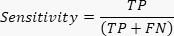
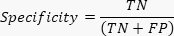
3. Use accuracy to report the overall correct classification rate. Use sensitivity to quantify disease-positive detection and specificity to quantify HC identification.
4. Use the F1 score to summarize the balance between precision and sensitivity. Use balanced accuracy to reduce the influence of class imbalance. In addition, compute the AUC to evaluate threshold-independent discrimination across decision thresholds.
5. For each repetition, average each performance metric across the five held-out folds. Report the final results as the mean and standard deviation of the 10 repetition-level means.
6. Compare BrainMoE with baseline methods. All baselines used the same participant-level partitions and full EEG-fMRI inputs as BrainMoE, with configurations fixed before held-out evaluation. BrainMoE was compared with each baseline using two-sided paired t-tests with Holm adjustment.

7. Perform group-level node occlusion attribution across five brain disorders

1. Define the attribution cohort. Load the trained BrainMoE checkpoint and the DK region name file. Select disease-positive test samples that are correctly classified under the full EEG-fMRI state with m = [1,1]. Use this cohort for group-level attribution analysis and save each sample's baseline target-disease probability.
2. Compute modality-specific node occlusion scores. For EEG-derived attribution, occlude one EEG ROI at a time by setting the selected EEG node feature vector and the corresponding row and column of the EEG graph to zero, while keeping the fMRI input unchanged. For fMRI-derived attribution, apply the same operation to the fMRI node feature matrix and fMRI graph, while keeping the EEG input unchanged. Repeat this procedure across all 68 DK regions. Run the node-occlusion attribution analysis using the code provided in Supplementary File 7.
3. Calculate and visualize group-level ROI contributions. For each ROI and each modality, calculate the contribution score as the mean decrease in target-disease probability after occlusion across all selected samples. Rank EEG-derived and fMRI-derived scores separately, export the top 10 ROIs for each modality, and label the highest-ranked ROI in the figure.

Results

BrainMoE performance across disorders and modality states
The protocol generated five disease-specific healthy-versus-disease BrainMoE classifiers and produced prediction tables for full EEG-fMRI, EEG-only, and fMRI-only inference states. The full EEG-fMRI state produced consistently high discrimination across the five tasks, with AUC values ranging from 84.4 ± 3.2% for RI to 88.4 ± 3.8% for ASD (Table 1). The macro-averaged full-state performance across the five tasks reached 86.9 ± 3.0% AUC, 81.4 ± 3.1% accuracy, 81.4 ± 2.5% balanced accuracy, and 81.2 ± 3.0% F1 score.

Under the simulated missing-modality conditions, BrainMoE maintained usable performance when one input modality was masked. In the EEG-only state, the model achieved a macro-averaged AUC of 83.1 ± 3.7%, with the strongest EEG-only AUC observed for ADHD at 87.9 ± 2.8%. In the fMRI-only state, the macro-averaged AUC was 80.0 ± 3.9%. These performance ranges and the expected full-state performance advantage serve as practical benchmarks for successful implementation, indicating that the trained BrainMoE framework can perform full, EEG-only, and fMRI-only inference without separate models for each modality.

A representative suboptimal outcome is failure to reproduce the expected full-state performance advantage, for example, when the full EEG-fMRI AUC is lower than the EEG-only or fMRI-only AUC. In contrast, successful implementation should reproduce the full-state advantage and the benchmark performance ranges reported in Table 1. When a suboptimal pattern is observed, verify the H5 input dimensions, the DK region order, the modality-availability mask assignment, and the saved cross-validation partitions before interpreting the model output.

Benchmark comparison
The proposed BrainMoE model was compared with classical machine learning methods (support vector machine (SVM) and multilayer perceptron (MLP)), general deep learning methods (Transformer⁷, 3D-CNN²² and ResNet⁶), advanced deep learning methods (BrainNetCNN⁸, BNT¹⁰, BrainGNN⁹, MultiEpilepsyNet¹¹, SZAtt-Net¹²), and MoE-based deep learning methods (dFCExpert¹⁷, EvoMoE¹⁸, and NeuroMoE++¹⁹) (Table 2). BrainMoE achieved the highest mean AUC among all methods compared, at 86.9 ± 3.0%.

Classical machine learning methods showed lower mean performance, with SVM achieving 66.7 ± 4.5% mean AUC and MLP 64.6 ± 6.3%. General deep learning methods showed variable performance, with ResNet achieving a mean AUC of 71.0 ± 3.3% and Transformer achieving 63.8 ± 4.7%. Among the advanced deep learning baselines, BNT, BrainGNN, MultiEpilepsyNet, and SZAtt-Net outperformed most classical and general deep learning methods, yet their mean AUCs remained lower than BrainMoE's.

To provide statistical support for the benchmark comparison, BrainMoE was compared with the strongest baseline for each performance metric (Table 3). BrainMoE outperformed NeuroMoE++ in AUC and balanced accuracy (BA) and outperformed SZAtt-Net in F1 score and accuracy. All comparisons remained significant after Holm adjustment.

Subgroup analysis by sex and acquisition site
Task-specific cohort characteristics, including the numbers of retained multimodal records, disease-to-control ratios, unique participant counts, age summaries, sex distributions, and acquisition-site distributions, are summarized in the cohort characteristics table (Table 4). The disease-to-control ratios are calculated from multimodal record counts, whereas demographic and acquisition-site characteristics are summarized at the unique-participant level.

To assess the potential effects of sex and acquisition site, BrainMoE performance was stratified by these factors (Table 5). The male subgroup showed higher mean AUC, BA, F1 score, and accuracy than the female subgroup, while the corresponding unadjusted Welch p values ranged from 0.089 to 0.321. Similarly, the RUBIC subgroup showed higher mean performance than the Staten Island subgroup, with p values ranging from 0.055 to 0.309. No statistically significant subgroup difference was detected in these analyses.

Ablation analysis of BrainMoE components
Ablation experiments were performed to assess the contribution of the modality availability mask, convolutional router, shared expert, and MoE expert fusion design (Table 6). Removing the mask embedding reduced the mean AUC to 79.2 ± 3.1%, and replacing the convolutional router with an MLP router reduced it to 79.3 ± 3.7%. Removing the shared expert reduced the fMRI-only AUC to 73.5 ± 3.3%, the lowest among the tested variants. Removing all MoE experts also reduced the overall balanced accuracy to 74.2 ± 3.0%. These ablation results showed that the full BrainMoE design achieved the strongest overall performance across both full- and missing-modality states, while the mask embedding, convolutional router, shared expert, and MoE expert fusion each contributed to the final model behavior.

ROI-level interpretability results for five brain disorders
To examine the regional contributions underlying BrainMoE predictions, node-occlusion attribution was performed on correctly classified disease-positive samples in the full EEG-fMRI state. EEG-derived and fMRI-derived ROI contributions were ranked separately by measuring the decrease in target-disease probability after occluding each DK atlas region. The analysis identified modality-specific contribution patterns across the five disease tasks (Figure 2). For fMRI-derived attribution, the top-ranked regions were the left posterior cingulate in MDD, the right pericalcarine cortex in ANX, the left parahippocampal cortex in RI, the right pars triangularis in ASD, and the left entorhinal cortex in ADHD. For EEG-derived attribution, the top-ranked regions were the left banks of the superior temporal sulcus in MDD, the left precentral cortex in ANX, the left cuneus in RI, the left lingual cortex in ASD, and the right insula in ADHD. The highest-ranked EEG- and fMRI-derived ROIs for each disorder are visualized on cortical surfaces in Figure 3. These results showed that BrainMoE provided ROI-level interpretability while preserving separate attribution profiles for EEG-derived and fMRI-derived representations. For correctly classified disease-positive samples, cross-fold stability was assessed using the Top-1 ROI frequency across 50 held-out folds (Table 7). The observed frequencies ranged from 36% to 68%, exceeding the theoretical random-selection reference of 1/68 (1.47%) and supporting interpretation based on relative rankings rather than absolute contribution magnitudes. Comparisons with previous neuroimaging findings were conducted post hoc and used only to contextualize the attribution results, not as independent validation.

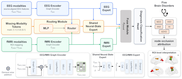
Figure 1: Overview of the BrainMoE framework with adaptive EEG-fMRI fusion for computer-assisted brain disorder diagnosis. Source-aligned EEG and fMRI ROI features are processed by separate Graph Encoders. The resulting representations are passed to the EEG and fMRI Experts and, together with the Modality Availability Mask, to the shared Soft-Routing Module. The modality representations and routing representation are fused and processed by the Shared neural-state expert. The three expert outputs are then combined in the Fuse Module and passed to the Diagnosis Classification Head to produce the HC and target-disease probabilities. Please click here to view a larger version of this figure.

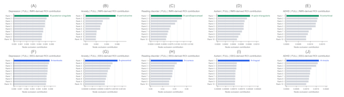
Figure 2: Node occlusion-based ROI contribution analysis. Top 10 EEG-derived and fMRI-derived ROI contributions were visualized for each disease task under the full EEG-fMRI inference state. Panels (A–E) show the fMRI-derived results for MDD, ANX, RI, ASD, and ADHD, respectively, and panels (F–J) show the corresponding EEG-derived results in the same order. Only the highest-ranked ROI was labeled in each plot. ROI contribution was defined as the decrease in target-disease probability after occluding the corresponding DK atlas region. Please click here to view a larger version of this figure.

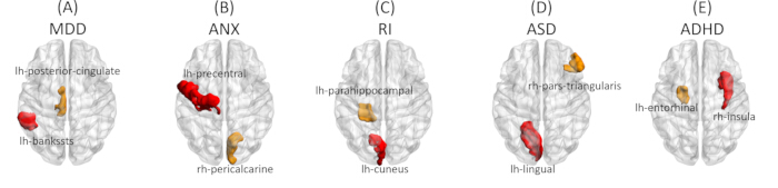
Figure 3: Cortical ROI-level interpretability maps across five brain disorders. Panels (A–E) show MDD, ANX, RI, ASD, and ADHD, respectively. Each panel displays the highest-ranked EEG-derived ROI in red and the highest-ranked fMRI-derived ROI in orange on the DK cortical surface. Colors indicate modality rather than contribution magnitude; therefore, no quantitative color scale is applied. The prefixes lh and rh denote the left and right hemispheres, respectively. Please click here to view a larger version of this figure.

Disease task	State	AUC	Accuracy	BA	F1	Sensitivity	Specificity
MDD	Full	88.0 ± 3.2%	84.8 ± 3.7%	82.0 ± 2.3%	76.2 ± 4.1%	72.7 ± 3.0%	91.3 ± 4.7%
MDD	EEG-only	83.4 ± 3.4%	81.8 ± 4.5%	77.9 ± 3.0%	73.7 ± 3.9%	68.2 ± 2.8%	87.6 ± 4.2%
MDD	fMRI-only	82.1 ± 3.3%	78.5 ± 4.7%	74.0 ± 4.1%	71.8 ± 4.9%	66.6 ± 3.5%	81.3 ± 5.6%
ANX	Full	85.5 ± 2.5%	76.1 ± 2.4%	78.2 ± 2.0%	79.4 ± 3.3%	78.1 ± 3.6%	78.2 ± 3.1%
ANX	EEG-only	81.7 ± 3.9%	73.2 ± 3.2%	75.6 ± 3.1%	78.1 ± 3.9%	76.6 ± 3.8%	74.6 ± 4.0%
ANX	fMRI-only	74.8 ± 4.1%	74.4 ± 3.7%	72.8 ± 3.6%	76.4 ± 4.2%	72.6 ± 3.9%	73.0 ± 4.4%
RI	Full	84.4 ± 3.2%	76.5 ± 3.0%	77.3 ± 2.9%	76.7 ± 2.8%	77.9 ± 3.1%	76.7 ± 3.3%
RI	EEG-only	80.2 ± 4.0%	71.5 ± 4.4%	73.4 ± 3.5%	73.0 ± 3.4%	73.8 ± 3.9%	72.9 ± 3.3%
RI	fMRI-only	81.3 ± 4.5%	71.1 ± 3.9%	67.9 ± 3.7%	68.5 ± 3.2%	69.4 ± 4.5%	66.3 ± 4.2%
ASD	Full	88.4 ± 3.8%	79.5 ± 3.5%	81.4 ± 3.0%	81.0 ± 2.8%	83.4 ± 2.9%	79.4 ± 3.0%
ASD	EEG-only	82.5 ± 4.3%	77.3 ± 4.1%	78.2 ± 3.7%	78.6 ± 3.5%	79.3 ± 3.4%	77.1 ± 4.1%
ASD	fMRI-only	81.3 ± 4.4%	73.8 ± 3.7%	74.4 ± 3.4%	75.0 ± 3.2%	76.1 ± 4.2%	72.6 ± 4.5%
ADHD	Full	88.2 ± 2.2%	90.3 ± 2.7%	88.4 ± 2.5%	92.8 ± 1.9%	87.0 ± 2.4%	89.7 ± 2.5%
ADHD	EEG-only	87.9 ± 2.8%	88.1 ± 2.6%	86.4 ± 3.1%	90.2 ± 3.4%	85.1 ± 3.1%	87.7 ± 3.0%
ADHD	fMRI-only	80.5 ± 3.2%	85.7 ± 3.0%	84.7 ± 3.5%	87.9 ± 4.1%	83.2 ± 3.6%	86.2 ± 3.4%

Table 1: BrainMoE classification performance across disease tasks and modality-availability states. Performance of BrainMoE for five healthy-versus-disease classification tasks under full EEG-fMRI, EEG-only, and fMRI-only inference states. Metrics are reported as mean ± standard deviation and include the area under the receiver operating characteristic curve (AUC), accuracy, balanced accuracy (BA), F1 score, sensitivity, and specificity.

Method	Method group	Mean AUC	Mean BA	Mean F1	Mean accuracy
SVM	Classical ML	66.7 ± 4.5%	70.6 ± 3.4%	61.7 ± 5.8%	70.7 ± 4.6%
MLP	Classical ML	64.6 ± 6.3%	63.5 ± 8.2%	64.5 ± 6.1%	64.2 ± 6.2%
Transformer	Generic DL	63.8 ± 4.7%	64.4 ± 4.8%	65.2 ± 5.1%	66.1 ± 4.9%
3D-CNN	Generic DL	65.3 ± 4.3%	65.2 ± 4.0%	64.8 ± 4.5%	60.0 ± 4.2%
ResNet	Generic DL	71.0 ± 3.3%	70.2 ± 3.6%	67.5 ± 3.8%	69.3 ± 3.0%
BrainNetCNN	Advanced DL	70.2 ± 3.6%	70.9 ± 3.1%	69.2 ± 3.6%	71.2 ± 3.1%
BNT	Advanced DL	73.6 ± 3.1%	76.4 ± 2.7%	74.7 ± 2.3%	76.6 ± 2.6%
BrainGNN	Advanced DL	72.4 ± 2.8%	72.7 ± 2.3%	71.0 ± 3.4%	72.3 ± 2.5%
MultiEpilepsyNet	Advanced DL	78.3 ± 3.7%	75.2 ± 3.5%	76.5 ± 3.6%	77.2 ± 3.3%
SZAtt-Net	Advanced DL	78.7 ± 3.2%	76.1 ± 3.8%	77.4 ± 3.9%	78.1 ± 3.4%
dFCExpert	MoE-based DL	80.1 ± 3.2%	77.3 ± 2.9%	76.7 ± 3.1%	77.6 ± 2.9%
EvoMoE	MoE-based DL	79.6 ± 3.6%	76.2 ± 3.1%	76.2 ± 3.3%	76.5 ± 3.2%
NeuroMoE++	MoE-based DL	81.5 ± 2.8%	77.9 ± 2.7%	77.1 ± 3.4%	78.0 ± 2.7%
BrainMoE (ours)	MoE-based DL	86.9 ± 3.0%	81.4 ± 2.5%	81.2 ± 3.0%	81.4 ± 3.1%

Table 2: Mean classification performance of BrainMoE compared with classical machine learning methods, generic deep learning models, and advanced neuroimaging deep learning architectures. Results are aggregated across the evaluated disease-classification tasks and reported as mean ± standard deviation for AUC, BA, F1 score, and accuracy.

Comparison	Mean AUC	Mean BA	Mean F1	Mean accuracy
Strongest baseline	NeuroMoE++	NeuroMoE++	SZAtt-Net	SZAtt-Net
Strongest-baseline performance	81.5 ± 2.8%	77.9 ± 2.7%	77.4 ± 3.9%	78.1 ± 3.4%
BrainMoE	86.9 ± 3.0%	81.4 ± 2.5%	81.2 ± 3.0%	81.4 ± 3.1%
Difference	+5.4	+3.5	+3.8	+3.3
t-test p	0.0006	0.0065	0.0187	0.0276
Holm-adjusted p*	p < 0.01	p < 0.05	p < 0.05	p < 0.05
Cohen's dz	1.63	1.11	0.91	0.83

Table 3: Comparison of BrainMoE with the strongest baseline for each performance metric. P values were calculated using two-sided paired t-tests and adjusted using the Holm procedure. Cohen's d_z denotes the standardized paired difference.

Cohort	Multimodal records (n)	Disease-to-control ratio	Unique participants (n)	Age range (years)	Sex (Male/Female)	Acquisition site (Staten Island/RUBIC)
HC	115	--	75	5.02–21.90	35/40	26/49
MDD	52	0.45:1	33	8.36–19.73	14/19	15/18
ANX	156	1.36:1	98	5.53–21.00	46/52	45/53
RI	141	1.23:1	85	5.75–19.66	47/38	39/46
ASD	82	0.71:1	51	5.66–19.79	45/6	27/24
ADHD	555	4.83:1	338	5.04–21.72	241/97	136/202

Table 4: Characteristics of the study cohorts used in the five disease-specific classification tasks. The table reports the number of retained multimodal records, disease-to-control ratios, unique participant counts, demographic characteristics, and acquisition-site distributions.

Subgroup	Number	Mean AUC	Mean BA	Mean F1	Mean accuracy
Sex
Male	705	87.2 ± 3.7	83.4 ± 3.2	82.1 ± 3.5	82.5 ± 3.8
Female	396	85.6 ± 3.3	81.2 ± 4.0	79.7 ± 3.8	79.6 ± 3.4
Difference		+1.6	+2.2	+2.4	+2.9
Welch p	--	0.321	0.192	0.159	0.089
Acquisition site
RUBIC	674	87.6 ± 4.0	83.3 ± 3.1	82.3 ± 3.7	83.4 ± 3.5
Staten Island	427	85.2 ± 3.6	81.7 ± 3.7	79.4 ± 3.4	80.1 ± 3.7
Difference		+2.4	+1.6	+2.9	+3.3
Welch p	--	0.176	0.309	0.085	0.055

Table 5: Sex- and acquisition-site-stratified performance of BrainMoE. Results are reported as mean ± standard deviation across 10 repetitions of 5-fold cross-validation. The difference represents the first subgroup minus the second, and P values were obtained using two-sided Welch t-tests.

Variant	Full AUC	EEG-only AUC	fMRI-only AUC	Mean AUC	Mean BA
w/o mask embedding	83.2 ± 2.9%	79.5 ± 3.9%	76.4 ± 3.7%	79.2 ± 3.1%	76.1 ± 3.4%
w/o Conv Router	84.6 ± 3.6%	80.7 ± 3.5%	78.2 ± 4.2%	81.6 ± 3.3%	75.7 ± 3.1%
MLP Router	82.8 ± 2.7%	80.1 ± 4.1%	76.6 ± 4.4%	79.3 ± 3.7%	74.1 ± 3.8%
w/o Shared Expert	83.3 ± 3.6%	80.8 ± 4.0%	73.5 ± 3.3%	80.1 ± 3.6%	75.5 ± 3.2%
w/o MoE Experts	81.9 ± 3.3%	78.7 ± 3.6%	78.0 ± 3.8%	80.8 ± 4.1%	74.2 ± 3.0%
BrainMoE (ours)	86.9 ± 3.0%	83.1 ± 3.7%	80.0 ± 3.9%	86.9 ± 3.0%	81.4 ± 2.5%

Table 6: Ablation analysis of key BrainMoE components. Ablation results showing the contribution of the modality availability mask, convolutional router, shared expert, and MoE expert-fusion design. Each variant is evaluated under full EEG-fMRI, EEG-only, and fMRI-only inference conditions, with mean AUC and mean BA summarizing overall performance.

Disease	EEG: top-ranked ROI	EEG: Top-1 frequency, n/N (%)	fMRI: top-ranked ROI	fMRI: Top-1 frequency, n/N (%)	Chance reference (%)
MDD	left banks of the superior temporal sulcus	22/50 (44%)	left posterior cingulate	25/50 (50%)	1.47
ANX	left precentral cortex	18/50 (36%)	right pericalcarine cortex	21/50 (42%)	1.47
RI	left cuneus	26/50 (52%)	left parahippocampal cortex	29/50 (58%)	1.47
ASD	left lingual cortex	27/50 (54%)	right pars triangularis	28/50 (56%)	1.47
ADHD	right insula	31/50 (62%)	left entorhinal cortex	34/50 (68%)	1.47

Table 7: Cross-fold stability of the top-ranked EEG- and fMRI-derived ROIs. Top-1 frequency denotes the number and percentage of 50-fold-level analyses in which the reported ROI ranked first. The theoretical random-selection reference was 1/68 (1.47%).

Supplemental File 1: H5 input-checking script. Python script for verifying the required H5 input keys, data types, diagnostic labels, and DK-atlas-compatible input dimensions before BrainMoE training. Please click here to download this file.

Supplemental File 2: fMRI preprocessing script. C-PAC configuration and execution files used for fMRI preprocessing, including initial-volume removal, motion and distortion correction, registration and normalization, nuisance regression, temporal filtering, and spatial smoothing. Please click here to download this file.

Supplemental File 3: FreeSurfer processing scripts. Scripts for processing structural MRI data, coregistering the Desikan-Killiany cortical parcellation to native fMRI space, and extracting ROI-level fMRI signals. Please click here to download this file.

Supplemental File 4: EEG preprocessing scripts. MATLAB/EEGLAB scripts used for EEG preprocessing, including filtering, artifact-component identification and removal, and rereferencing. Please click here to download this file.

Supplemental File 5: MNE-Python source-localization and feature-extraction script. Python script for EEG source localization, DK-atlas ROI extraction, and generation of ROI-level EEG features used as BrainMoE inputs. Please click here to download this file.

Supplemental File 6: BrainMoE implementation code. Python code and configuration files for the BrainMoE architecture, graph encoders, modality-state handling, expert routing and fusion, model training, evaluation, and ablation variants. Please click here to download this file.

Supplemental File 7: Node-occlusion attribution code. Python code for modality-specific node-occlusion analysis, calculation of ROI contribution scores, ranking of EEG- and fMRI-derived ROIs, and generation of attribution outputs. Please click here to download this file.

Discussion

Multimodal brain signal analysis has become an important direction for computer-assisted brain disorder diagnosis because EEG and fMRI provide complementary information about neural activity. In the benchmark comparison, classical machine learning methods such as SVM and MLP delivered basic diagnostic performance but had limited ability to model hierarchical, graph-structured, and cross-modal feature interactions. Generic deep learning models, including 3D-CNN, ResNet, and Transformer, offered stronger nonlinear modeling capacity, but these architectures were not specifically designed for EEG-fMRI fusion or brain network representations. Advanced deep learning methods achieved better performance than most classical and generic models, but many still relied on fixed feature-integration strategies and did not explicitly separate modality-specific information from shared neural-state information.

This study proposed BrainMoE to address this fusion problem by combining graph-based modality encoders, modality-specific experts, a shared neural-state expert, and an adaptive routing mechanism. This design allowed EEG-derived and fMRI-derived representations to be modeled separately and then integrated through expert-level fusion. By introducing modality-state masks and missing-modality tokens, the same trained model could also perform EEG-only and fMRI-only inference without constructing separate models for each missing-modality condition. The experimental results showed that BrainMoE achieved the strongest overall performance across the five binary disease classification tasks, and maintained usable performance under both EEG-only and fMRI-only states. The ablation analysis further supported the contribution of the mask embedding, convolutional router, shared expert, and MoE expert fusion. These findings indicate that the improved performance was not due to a single component, but to the coordinated design of graph encoding, modality-state modeling, adaptive routing, and expert fusion.

Critical protocol steps and troubleshooting
Critical protocol steps include maintaining the same 68-region DK order across the EEG and fMRI node and graph matrices, applying the predefined preprocessing settings independently for each participant, and enforcing participant-level cross-validation so that all records from the same participant remain in a single fold. The Modality Availability Mask must also correspond to the supplied inputs for each inference state.

If inference fails or the expected full-state performance advantage is not reproduced, first verify the required H5 keys, the EEG and fMRI matrix dimensions, the DK region order, the Modality Availability Mask assignment, and the saved cross-validation partitions. Files with missing keys, invalid dimensions, or inconsistent region ordering should be excluded before training or evaluation. The framework can be modified for alternative cortical parcellations or EEG/fMRI feature representations, provided that both modalities are mapped to a consistent ROI ordering and the corresponding model input dimensions are adjusted. The disease-specific classification head can also be adapted to other binary classification tasks while retaining the graph-encoding and expert-fusion framework. Such modifications require retraining and validation rather than direct application of the models reported here.

Node occlusion-based interpretability analysis
The node-occlusion analysis further provided ROI-level interpretability of the BrainMoE predictions, with the top-ranked disease-associated ROIs shown in Figure 3. The EEG-derived left posterior ROI identified by BrainMoE is consistent with prior voxel-based meta-analytic²³ evidence reporting altered intrinsic brain activity in posterior cortical regions in MDD. The EEG/fMRI-derived left precentral and right pericalcarine ROIs are consistent with previous neuroimaging evidence in anxiety disorders: a cortical-thickness meta-analysis²⁴ reported increased cortical thickness in the left precentral gyrus in patients with anxiety disorders, while a structural covariance network study²⁵ in social anxiety disorder reported abnormal nodal centrality involving the right pericalcarine cortex. For reading disorder, the EEG-derived left cuneus ROI is consistent with a whole-brain connectivity study²⁶ reporting altered left cuneus connectivity in dyslexia, whereas the fMRI-derived left parahippocampal ROI is consistent with a separate study²⁷ reporting abnormal parahippocampal/hippocampal coupling in adolescents with specific reading comprehension deficits. In the autism spectrum disorder task, the left lingual ROI highlighted by EEG-derived attribution echoes prior resting-state fMRI evidence²⁸ of reduced ReHo in the left lingual gyrus in prepubertal boys with ASD. The fMRI-derived right pars triangularis ROI is also biologically plausible, as altered ALFF in the right pars triangularis of the inferior frontal gyrus has been reported²⁹ in autistic children. For ADHD, the EEG-derived right insula ROI fits with structural MRI evidence³⁰ showing reduced anterior insular volume in youths with ADHD, particularly involving the right insular short gyrus. The fMRI-derived left entorhinal ROI may reflect a more subtype-specific finding, as a separate Psychological Medicine study³¹ reported lower left entorhinal cortex volume in an ADHD-C subgroup after FDR correction. These findings should nevertheless be interpreted with consideration of interregional dependence, because correlated ROI signals may prevent single-node occlusion from fully isolating an individual region's contribution and may lead to conservative estimates.

Limitations and future directions
Although repeated 5-fold cross-validation was used to obtain internal performance estimates, future studies using nested cross-validation or independent external validation would further strengthen the assessment of model-selection stability and generalizability. Because the EEG-only and fMRI-only outputs were generated by masking one modality in complete multimodal records and were not evaluated on an external validation cohort, future studies should include external single-modality validation cohorts to assess generalizability. A further limitation is that the healthy-versus-single-disease design does not capture comorbid presentations, which limits clinical generalizability and motivates future studies of multi-label classification and differential diagnosis. Future work could also evaluate the robustness of source-level EEG associations using leakage-aware connectivity estimators. Although the shared DK parcellation provides an anatomically grounded interface for multimodal fusion, it is a modeling assumption that may not fully capture modality-specific differences in temporal resolution and physiological origin. Beyond the five disorders evaluated here, the framework could be adapted to other neurological or psychiatric classification tasks involving anatomically aligned multimodal brain data and extended to multi-label or differential-diagnosis applications.

Conclusion
In summary, BrainMoE provides a practical and interpretable framework for EEG-fMRI fusion in computer-assisted diagnosis of brain disorders. Its main advantage lies in adaptive multimodal feature integration, driven by a multi-expert architecture and a soft-routing mechanism that dynamically balances modality-specific and shared information. Furthermore, by seamlessly incorporating modality-state masks and missing-modality tokens, the same trained model achieves robust performance during incomplete-modality inference without requiring separate configurations. Crucially, the interpretable framework provides transparent, group-level regional attribution pathways across five distinct brain disorders, transforming the conventional black-box architecture into a physiologically informed tool for computer-assisted diagnosis. This is important for future computational neuroimaging workflows in which heterogeneous data sources, incomplete modality availability, and explainable model outputs are all central considerations.

Materials

List of materials used in this article

Name	Company	Catalog Number	Comments
Bash	GNU Project	5.1.16(1)-release	Software
C-PAC	FCP-INDI	Version 1.8.7; container tag release-v1.8.7.dev1	Software
CUDA Toolkit	NVIDIA Corporation	Version 12.4	Software
CUDA-compatible GPU	NVIDIA Corporation	GeForce RTX 4060 Laptop GPU	Equipment
Desikan-Killiany cortical atlas	FreeSurfer, Athinoula A. Martinos Center for Biomedical Imaging, Massachusetts General Hospital	aparc; 68 cortical regions (RRID:SCR_001847)	Atlas/resource
EEGLAB	Swartz Center for Computational Neuroscience, University of California San Diego	Version 2022.1 (RRID:SCR_007292)	Software
FreeSurfer	Athinoula A. Martinos Center for Biomedical Imaging, Massachusetts General Hospital	Version 7.4.1 (RRID:SCR_001847)	Software
FSL	FMRIB, University of Oxford	Bundled with C-PAC 1.8.7; exact version not specified (RRID:SCR_002823)	Software
Healthy Brain Network (HBN) dataset	Child Mind Institute	RRID:SCR_016989	Dataset
MATLAB	MathWorks	R2022a (RRID:SCR_001622)	Software
MNE-Python	MNE-Python Development Team	Version 1.9 (RRID:SCR_005972)	Software/library
Python	Python Software Foundation	Version 3.12.4 (RRID:SCR_008394)	Software
PyTorch	PyTorch Foundation	Version 2.6.0+cu124 (RRID:SCR_018536)	Library

References

- Shao Y, et al. Exploring cognitive workload recognition using CogRepLKNet with EEG-fMRI. Neural Netw. 2026;198:108575.
- Jatoi MA, et al. A survey of methods used for source localization using EEG signals. Biomed Signal Process Control. 2014;11:42-52.
- Wei X, et al. Multi-modal cross-domain self-supervised pre-training for fMRI and EEG fusion. Neural Netw. 2025;184:107066.
- Lang J, Yang LZ, Li H. Multi-modal dynamic brain graph representation learning for brain disorder diagnosis via temporal sequence model. Neurocomputing. 2025;656:131509.
- Zhu W, et al. CGLK-GNN: a connectome generation network with large kernels for GNN based Alzheimer's disease analysis. Neural Netw. 2026;199:108689.
- Wu Z, Shen C, van den Hengel A. Wider or deeper: revisiting the ResNet model for visual recognition. Pattern Recogn. 2019;90:119-33.
- Vaswani A, et al. Attention is all you need [conference paper]. Presented at: 31st Conference on Neural Information Processing Systems; Long Beach, CA; 2017. Available from: https://papers.nips.cc/paper/7181-attention-is-all-you-need
- Kawahara J, et al. BrainNetCNN: convolutional neural networks for brain networks; towards predicting neurodevelopment. Neuroimage. 2017;146:1038-49.
- Li X, et al. BrainGNN: interpretable brain graph neural network for fMRI analysis. Med Image Anal. 2021;74:102233.
- Kan X, et al. Dynamic brain transformer with multi-level attention for functional brain network analysis [conference paper]. Presented at: 2023 IEEE EMBS International Conference on Biomedical and Health Informatics; Pittsburgh, PA; 2023. Available from: https://doi.org/10.1109/BHI58575.2023.10313480
- Khan MAR, et al. MultiEpilepsyNet: an EEG and MRI data based multimodal seizure detection model using hybrid deep learning model. Brain Res Bull. 2025;233:111645.
- Saha A, Ghosh D, Ali F, Singh PK. SZAtt-Net: a unified deep learning model with different attention mechanisms for schizophrenia classification from multimodal data. Med Nov Technol Devices. 2026;29:100428.
- Liu J, et al. A survey on inference optimization techniques for mixture of experts models. ACM Comput Surv. 2026;58(10):1-37.
- Xu H, et al. MCMoE: completing missing modalities with mixture of experts for incomplete multimodal action quality assessment [conference paper]. Presented at: 40th Annual AAAI Conference on Artificial Intelligence; Singapore; 2026. Available from: https://doi.org/10.1609/aaai.v40i13.38104
- Nguyen H, Ho N, Rinaldo A. Convergence rates for softmax gating mixture of experts. IEEE Trans Inf Theory. 2025;72(2):1276-304.
- Ma J, et al. Modeling task relationships in multi-task learning with multi-gate mixture-of-experts [conference paper]. Presented at: 24th ACM SIGKDD International Conference on Knowledge Discovery & Data Mining; London, United Kingdom; 2018. Available from: https://doi.org/10.1145/3219819.3220007
- Chen T, Li H, Zheng H, Fan Y. dFCExpert: learning dynamic functional connectivity patterns with modularity and state experts. IEEE Trans Med Imaging. 2026;45(3):1088-98.
- Yang X, et al. EvoMoE: evolutionary mixture-of-experts for SSVEP-EEG classification with user-independent training. IEEE J Biomed Health Inform. 2025;29(9):6538-50.
- Raza WH, et al. NeuroMoE++: patient-adaptive multi-level multimodal fusion with mixture-of-experts for neurological disorder classification. IEEE Trans Biomed Eng. 2026;73(8):2784-94.
- Desikan RS, et al. An automated labeling system for subdividing the human cerebral cortex on MRI scans into gyral based regions of interest. Neuroimage. 2006;31(3):968-80.
- Alexander LM, et al. An open resource for transdiagnostic research in pediatric mental health and learning disorders. Sci Data. 2017;4(1):170181.
- Ji S, Xu W, Yang M, Yu K. 3D convolutional neural networks for human action recognition. IEEE Trans Pattern Anal Mach Intell. 2013;35(1):221-31.
- Gong J, et al. Common and distinct patterns of intrinsic brain activity alterations in major depression and bipolar disorder: voxel-based meta-analysis. Transl Psychiatry. 2020;10(1):353.
- Wang L, et al. Alterations in cortical thickness in anxiety disorders and their association with atlas-based neurotransmitter maps. Acad Radiol. 2026;33(7):3011-22.
- Zhang X, et al. Disrupted brain gray matter connectome in social anxiety disorder: a novel individualized structural covariance network analysis. Cereb Cortex. 2023;33(16):9627-38.
- Finn ES, et al. Disruption of functional networks in dyslexia: a whole-brain, data-driven analysis of connectivity. Biol Psychiatry. 2014;76(5):397-404.
- Cutting LE, et al. Not all reading disabilities are dyslexia: distinct neurobiology of specific comprehension deficits. Brain Connect. 2013;3(2):199-211.
- Yue X, et al. Brain functional alterations in prepubertal boys with autism spectrum disorders. Front Hum Neurosci. 2022;16:891965.
- Karavallil Achuthan S, Coburn KL, Beckerson ME, Kana RK. Amplitude of low frequency fluctuations during resting state fMRI in autistic children. Autism Res. 2023;16(1):84-98.
- Lopez-Larson MP, et al. Reduced insular volume in attention deficit hyperactivity disorder. Psychiatry Res Neuroimaging. 2012;204(1):32-9.
- Yamashita M, Shou Q, Mizuno Y. Unsupervised machine learning for identifying attention-deficit/hyperactivity disorder subtypes based on cognitive function and their implications for brain structure. Psychol Med. 2024;54(14):3917-29.
Reprints and Permissions
This article has been published
Video Coming Soon