Este protocolo describe métodos para generar pececitos cebra transgénicos compuestos, obtener imágenes de células inmunitarias asociadas con tumores en pececitos cebra larvales y adultos, y cuantificar la frecuencia de células inmunitarias dentro del microambiente tumoral.
Artículo de método
Imagen y cuantificación de células inmunitarias en el microambiente tumoral utilizando un modelo de neuroblastoma en pez cebra
* These authors contributed equally
En este artículo
Resumen
Resumen
La reclutación de células inmunitarias hacia el microambiente tumoral (TME) es un componente importante de la regulación inmunitaria y la progresión tumoral. El estudio de las relaciones espaciales y temporales entre células inmunitarias y tumorales in vivo puede proporcionar información sobre las interacciones que ocurren dentro del TME. Sin embargo, visualizar y cuantificar estas interacciones en organismos intactos sigue siendo un desafío con los enfoques convencionales de imagen y histología. Los peces cebra constituyen un modelo valioso para la investigación del cáncer debido a su facilidad genética, desarrollo rápido y transparencia óptica durante las etapas tempranas del desarrollo, lo que permite la visualización de células marcadas con fluorescencia in vivo. Aquí presentamos un protocolo para generar, identificar, visualizar y cuantificar células inmunitarias y tumorales marcadas diferencialmente con marcadores fluorescentes en un modelo de pez cebra de neuroblastoma. El protocolo incluye el cruce y cribado de peces cebra transgénicos compuestos, la imagen en vivo de larvas, la preparación y visualización de peces adultos portadores de tumores, y la cuantificación de células inmunitarias que rodean y se encuentran dentro de las regiones tumorales. Mediante líneas transgénicas con reporteros, CD4+ células inmunitarias y MYCNcélulas de neuroblastoma impulsadas por pueden visualizarse y analizarse en diferentes etapas del desarrollo. El flujo de trabajo permite la evaluación de la localización de las células inmunitarias en relación con los tumores tanto en peces larvales como adultos, y puede utilizarse para comparar la abundancia de células inmunitarias entre distintas etapas de la enfermedad. Este protocolo proporciona un enfoque reproducible para la obtención de imágenes y la cuantificación de células inmunitarias dentro del microambiente tumoral (TME) in vivo utilizando peces cebra y podría facilitar estudios de las interacciones inmune-tumor en otros modelos de cáncer.
Introducción
El microambiente tumoral (TME) es un ecosistema compuesto por células tumorales, inmunitarias, fibroblastos y células vasculares1. El TME desempeña un papel esencial en la progresión del cáncer, la respuesta terapéutica y la inmunidad antitumoral. Dentro del TME, las células inmunitarias son reguladores clave del destino tumoral, ya sea participando en respuestas antitumorales o induciendo inmunosupresión2. Comprender el reclutamiento, la distribución y la función de las células inmunitarias dentro del TME es fundamental para elucidar los mecanismos mediante los cuales los tumores evaden la vigilancia inmunitaria. Sin embargo, los enfoques convencionales para estudiar el TME, como la histología de punto final, la citometría de flujo y la secuenciación de células individuales, solo proporcionan imágenes estáticas y a menudo requieren la interrupción de la estructura del tejido, lo que resulta en la pérdida de información espacial y de interacciones célula-célula3,4,5,6,7. Además, estos métodos tienen limitaciones en su capacidad para visualizar y cuantificar células inmunitarias dentro del TME, especialmente durante las primeras etapas del desarrollo tumoral.
Los peces cebra (Danio rerio) son un modelo potente para la investigación del cáncer debido a su bajo costo, desarrollo rápido, transparencia relativa y alta conservación genética8,9. Estas ventajas proporcionan un sistema experimental reproducible y escalable que permite tamaños grandes de muestra y cribado eficiente mediante microscopía en un período corto de tiempo10. Es importante destacar que los peces cebra comparten una conservación inmunológica significativa con los seres humanos, incluyendo componentes clave tanto del sistema inmunitario innato como del adaptativo, lo que hace que los hallazgos sean relevantes para enfermedades humanas11. Estas propiedades son particularmente útiles para estudiar cánceres pediátricos como el neuroblastoma8. En consecuencia, se han desarrollado numerosas líneas de reportero inmunitario y modelos de cáncer en pez cebra11. Por lo tanto, el pez cebra sirve como un modelo valioso in vivo para estudiar las interacciones entre células tumorales e inmunitarias, ofreciendo información sobre cómo la regulación inmunitaria influye en el desarrollo tumoral, especialmente durante las etapas iniciales.
Estudios previos que investigan el MTE en pez cebra han dependido en gran medida de modelos de xenoinjertos tumorales combinados con imágenes de punto final para evaluar la localización de células inmunitarias dentro de los tumores12,13,14,15,16,17. Aunque estos métodos proporcionan información útil, están limitados por su dependencia de imágenes bidimensionales, que no pueden capturar completamente la organización tridimensional del MTE ni las relaciones espaciales entre células tumorales e inmunitarias durante el desarrollo14. Además, los modelos de xenoinjerto tumoral implican el trasplante artificial de células tumorales humanas y pueden no recapitular completamente la iniciación tumoral natural18. Estos modelos también son generalmente a corto plazo y no pueden capturar completamente la progresión tumoral ni los cambios en la relación espacial entre células tumorales e inmunitarias durante el desarrollo14,19. Asimismo, este enfoque ofrece una representación limitada de la organización espacial, el contexto de desarrollo y la relevancia fisiológica del comportamiento de las células inmunitarias dentro del MTE. Recientemente, nosotros y otros investigadores hemos aplicado peces cebra transgénicos compuestos, en los cuales las células tumorales e inmunitarias están marcadas diferencialmente con indicadores fluorescentes, para visualizar células inmunitarias asociadas con tumores20,21. Estos peces transgénicos compuestos permiten el estudio del MTE a lo largo del desarrollo del animal y del tumor, facilitando investigaciones sobre las interacciones entre el sistema inmunitario y el tumor in vivo.
Aquí, presentamos un método que utiliza microscopía confocal para estudiar las células inmunitarias dentro del microentorno tumoral (TME) de un modelo de neuroblastoma en pez cebra. En este enfoque, utilizamos líneas reporteras de pez cebra que marcan las células inmunitarias y una línea de pez cebra genéticamente modificada que sobreexpresa el oncogén humano MYCN bajo el promotor de dopamina-β-hidroxilasa (dβh), lo que resulta en el desarrollo de neuroblastoma que se asemeja a la enfermedad humana20. En este modelo transgénico compuesto, las células tumorales e inmunitarias se marcan diferencialmente con EGFP y mCherry, respectivamente. El promotor dβh está activo en las células de la línea simpaticoadrenal y se ha utilizado en múltiples modelos de pez cebra de neuroblastoma22,23,24,25. Además, utilizamos un promotor Cd4 que induce la fluorescencia de mCherry para visualizar las células CD4+15. Se aplicó la adquisición de imágenes confocales con Z-stacks para visualizar el TME en tres dimensiones en diferentes etapas del desarrollo tumoral, permitiendo evaluar las relaciones espaciales entre las células tumorales e inmunitarias dentro del tejido intacto. Este método permite analizar la organización de las células inmunitarias respecto a las células tumorales durante distintas etapas del desarrollo tumoral.
Protocolo
All animal procedures were approved by the Institutional Animal Care and Use Committee (IACUC) at Boston University Chobanian & Avedisian School of Medicine under protocol PROTO202100001. The overall workflow for generation of compound transgenic zebrafish, larval imaging, adult tissue preparation, and image analysis is summarized in Figure 1.
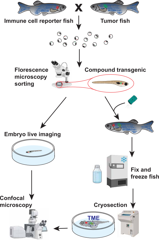
Figure 1. Workflow for visualization and quantification of immune cells within the zebrafish tumor microenvironment (TME). Schematic overview of the experimental workflow. Immune-reporter zebrafish were crossed with tumor-prone zebrafish to generate compound transgenic offspring expressing fluorescent markers in both immune cells (red) and tumor cells (green). Embryos were screened by fluorescence microscopy to identify compound transgenic fish. Selected fish were either subjected to live confocal imaging during larval development (<21 days post-fertilization [dpf]) or processed by fixation, cryosectioning, and confocal imaging for fish older than 21 dpf. This workflow enables visualization and quantification of immune cells associated with the TME across multiple developmental stages. Part of the illustration was created using BioRender. Please click here to view a larger version of this figure.
1. Generation of Compound Transgenic Zebrafish Lines Through Breeding
- Select adult immune-reporter fish and tumor fish that are at least 3 months old for natural breeding.
NOTE: For the representative results, Tg(cd4-1:mCherry) heterozygous fish were crossed with Tg(dβh:MYCN; dβh:EGFP) heterozygous fish to differentially label immune cells and tumor cells15,23. - On the evening before breeding, fill a two-chamber mating tank two-thirds full with fish water.
- Place a grated top insert into the mating chamber. Use dividers to separate one male from one or two females.
- Leave the dividers in place overnight. Add artificial plants or other enrichment items to simulate natural breeding conditions.
NOTE: A 1:2 male-to-female ratio increases the likelihood of successful spawning when breeding tumor male fish with immune-reporter fish. Do not breed two males with one female, as competition between males may occur. - On the following morning, remove the dividers after the facility lights turn on.
- Tilt the grated top chamber slightly using the divider as a wedge to create a shallow water area. Allow the fish to spawn for at least 1 h.
- Collect eggs from the bottom of the mating chamber by pouring the water through a fine-mesh net.
- Transfer the eggs to a sterile Petri dish containing fish water at a density no greater than 1 egg per 50 mm2 (approximately 200 eggs per 100 mm dish).
- Remove dead and unfertilized eggs.
NOTE: Healthy fertilized eggs are translucent and round. Remove cloudy, white, unfertilized, or deformed eggs. - Double-check the fish to avoid mixing sexes or cross-contaminating transgenic tanks.
- Return the males and females to their respective tanks.
- Place the embryos in a 28.5°C incubator overnight. Do not exceed the embryo density specified in Step 1.8.
- Bleach the embryos on the following morning to remove contaminants.
- Prepare a working bleach solution consisting of 100 µL bleach in 200 mL system water. Prepare a neutralization solution consisting of 0.5 g sodium thiosulfate in 150–200 mL system water.
- Sort and transfer viable embryos into a mesh-net well insert. Submerge the insert in the bleach solution for 5 min.
- Transfer the insert directly into the sodium thiosulfate solution. Incubate for 2 min to neutralize residual bleach.
- Rinse the embryos in a final bath of fresh system water. Use a squirt bottle to gently transfer the embryos into clean petri dishes containing fresh system water.
- Return the embryos to the incubator after bleaching.
- Transfer larvae at 5–7 days post-fertilization (dpf) or later to a larger tank containing 5 ppt rotifer water for rearing.
- Prepare 5 ppt rotifer water by mixing 1 part stock rotifer water (15 ppt) with 2 parts zebrafish system water.
- Verify that the final salinity is 5 ppt using a conductivity meter before transferring the larvae.
NOTE: Sorting EGFP+ MYCN larvae at 3–5 dpf facilitates identification of tumor-prone fish before rearing. Sorting MYCN embryos at this stage avoids false-negative identification because EGFP expression in neural crest cells may decrease later in development due to MYCN-induced apoptosis.
2. Screening Zebrafish for Fluorescent Markers
- Prepare a 0.4% (w/v) tricaine stock solution using system water.
- Transfer the fish to a clean petri dish containing only enough system water to cover the bottom.
- Add the tricaine stock solution to achieve a final concentration of approximately 0.005% (50 mg/L) for fish younger than 14 dpf or 0.012% (120 mg/L) for fish older than 14 dpf. Confirm adequate anesthesia by observing little to no voluntary movement.
- Remove excess water from the dish once the fish are anesthetized and no longer capable of swimming while maintaining visible opercular or cardiac movement.
- Screen the fish for fluorescence. Identify green or red fluorescence in the expected region (e.g., the interrenal gland region in MYCN fish).
- Separate the fish into groups using a stiff-bristled sorting tool.
NOTE: Sort tumor-prone fish as early as possible because MYCN-induced apoptosis during later developmental stages may result in false-negative identification. Sort immune-reporter fish immediately before imaging at the larval stage or between 2 and 4 months of age for adult studies. This approach minimizes handling-associated stress and maximizes survival. - Transfer positive and negative fish to separate tanks containing system water for continued rearing.
NOTE: Step 3 describes handling and imaging of larvae younger than 21 dpf. Steps 4–6 describe fixation, tissue preparation, imaging, and image analysis of older fish.
3. Larval Live-Mounting and Imaging
- Place sorted larvae in a 100 mm petri dish containing tricaine fish water (see Step 2.3 for age-appropriate concentrations).
- Transfer the sedated larvae to a glass-bottom imaging dish.
- Use only enough solution to cover the larva and maintain sedation.
- Prepare 1%–1.5% low-melting agarose in fish water. Heat the agarose solution until fully dissolved.
- Allow the agarose to cool for 1–2 min. Maintain the agarose at 30°C using a heat block to prevent solidification prior to mounting.
- Position each larva laterally in the imaging dish.
- Apply approximately 30–200 µL of agarose over the larva to immobilize it. Use larger volumes for larger larvae and smaller volumes for smaller larvae.
- Once the agarose has solidified, add approximately 100 µL of 0.005% tricaine solution over the agarose.
- Image the larvae using a confocal microscope.
- Use a standard laser-scanning confocal microscope with a resonant scanner. Use a 40× objective with a numerical aperture greater than 1.10.
- Set the pinhole to 1.0 Airy unit (AU) for all imaging channels.
- Use a 488 nm laser for EGFP excitation and a 594 nm laser for mCherry excitation. Keep laser output below 25 mW to minimize photobleaching and phototoxicity. Adjust detector gain and laser power using a range indicator lookup table (LUT) to avoid pixel saturation and black clipping. Do not exceed a detector gain of 800 V because higher voltages introduce excessive noise.
- Use a voxel size of 0.42 × 0.42 × 6.0 µm (x, y, z) at a resolution of 1024 × 1024 pixels and a Z-step interval of 6.0 µm. Acquire optical sections continuously through the full volume of interest, typically spanning 90–120 µm in total imaging depth. Use highly sensitive photodetectors operating in 16-bit acquisition mode.
- Acquire images using unidirectional line scanning at a resonant scan frequency of 33.3 kHz (approximately 1.58 µs pixel dwell time). Use 2× or 4× averaging to reduce motion artifacts while limiting laser exposure.
NOTE: Optimize tricaine exposure to maintain larval survival during imaging. After imaging, add fish water until the imaging dish is approximately half full.
- Add fresh fish water to the imaging dish immediately after imaging.
- Gently remove the larva from the agarose using a stiff-bristled stick and transfer the larva to a dish containing clean fish water for recovery.
- Return the fish to its original tank once normal swimming behavior resumes.
NOTE: For fish older than 21 dpf, the skin overlying the tumor must be removed by cryosectioning to enable high-resolution confocal imaging.
4. Fish Fixation and Cryosectioning
- Euthanize fish in accordance with approved institutional animal care guidelines.
- Make a ventral incision extending from the anal pore to the pectoral girdle to expose the abdominal cavity and facilitate fixative penetration into internal tissues.
- Transfer the fish using forceps into a 1.5 mL tube containing 4% paraformaldehyde (PFA) in phosphate-buffered saline (PBS) or a volume of fixative at least 10-fold greater than the tissue volume.
NOTE: Avoid handling the region containing the tumor to preserve tissue integrity. - Place the samples on a nutating rocker set to gentle continuous agitation (30 rpm) and incubate overnight for at least 12 h at 4°C.
CAUTION: PFA is hazardous, toxic, and potentially carcinogenic. Wear appropriate personal protective equipment, including gloves and eye protection. Perform all procedures involving PFA in a fume hood and avoid inhalation of vapors. - Remove the PFA and wash the samples at least four times with 1.5 mL of 1× PBS. Gently invert the tube two to three times during each wash.
- Transfer the fish to 30% sucrose prepared in PBS.
- Incubate the fish in a cold room overnight until the specimen sinks to the bottom of an upright tube (approximately 12 h), indicating adequate sucrose penetration.
- Remove excess sucrose solution by gently blotting the fish on a laboratory tissue.
- Transfer the fish to storage tubes.
- Store the samples at −80°C until imaging.
NOTE: Process samples within 3 months to minimize fluorescent protein degradation and signal loss. - Transport the fixed fish to the cryostat room on dry ice.
- Place the fish flat in a plastic mold with one sagittal side facing downward.
- Add Optimal Cutting Temperature (OCT) compound until the fish is fully covered.
- Freeze the mold at −20°C or in the cryostat until the OCT turns white.
NOTE: Position the fish as flat as possible before freezing to facilitate consistent sectioning. - Cryosection the zebrafish in the sagittal plane to remove the skin for subsequent whole-mount imaging.
- Cool the cryostat chuck.
- Apply room-temperature OCT to the chuck.
- Press the OCT fish block firmly into the OCT layer.
- Freeze the chuck and block until the newly applied OCT turns white.
- Mount the chuck in the cryostat.
- Cryosection the block at a thickness of 14 µm until the blade reaches the specimen.
NOTE: Specimen shifting may occur during freezing, causing the fish to sit higher in the block than expected. Entry into the specimen is indicated by the appearance of translucent tissue replacing the opaque OCT background. - Reduce the section thickness to 7 µm.
- Continue sectioning for one additional cut.
NOTE: This procedure removes the skin while preserving a uniform sagittal profile across the specimen. - Confirm the endpoint by identifying skin in the collected sections.
NOTE: Skin appearance in sections provides a more reliable indicator than eye morphology. Perform this procedure only when the skin obscures imaging of the tumor microenvironment.
- Warm the chuck gently with your hands.
- Remove the OCT block from the chuck using forceps. Avoid disturbing the cut surface of the specimen.
- Trim excess OCT surrounding the fish while the OCT remains frozen.
- Remove the fish from the OCT block using forceps once the OCT softens to a viscous consistency.
5. Mounting and Imaging of Fish with Skin Removed
- Place the fish in a glass-bottom dish with the sectioned sagittal side facing the glass surface.
NOTE: Maintain the orientation of the fish during handling. Identifying the sectioned side may become difficult after the fish is removed from the OCT block. - Prepare 1%–1.5% low-melting agarose.
- Apply approximately 30–50 µL of agarose to the dorsal and ventral sides of the fish to secure the sample.
NOTE: Avoid placing agarose beneath the fish because it can reduce image quality. Use only the minimum amount of agarose required for stabilization. - Keep the sample on ice during transport. Image the sample within 2 h of mounting.
- Transport the sample to the confocal microscopy facility.
- Image the sample using confocal microscopy.
- Use a standard laser-scanning confocal microscope with a resonant scanner. A two-photon microscope may be used when autofluorescence limits image quality. Use a corrected 20× objective lens with a numerical aperture of at least 0.80.
- Set the pinhole to 1.0 Airy unit (AU) for all imaging channels.
- Use a 488 nm laser for EGFP excitation and a 594 nm laser for mCherry excitation. Keep laser output below 25 mW. Adjust detector gain and laser power using a range indicator lookup table (LUT) to avoid pixel saturation and black clipping. Do not exceed a detector gain of 800 V because higher voltages introduce excessive noise.
- Configure image acquisition parameters as follows.
- Use a voxel size of 0.42 × 0.42 × 6.0 µm (x, y, z) at a resolution of 1024 × 1024 pixels and a Z-step interval of 6.0 µm.
- Acquire spectral image stacks through the full volume of interest, typically spanning a total Z-stack acquisition range of 90–120 µm (15–20 optical sections).
- Initiate image acquisition in the fluid space immediately above the tissue surface and continue through the full target imaging depth to ensure complete coverage of the specimen.
- Acquire images using highly sensitive photodetectors operating in 16-bit acquisition mode.
- Acquire images using unidirectional line scanning at a resonant scan frequency of 33.3 kHz (approximately 1.58 µs pixel dwell time) with 8× line averaging.
6. Image Analysis and Quantification
- Image visualization using Fiji (version 1.54p).
- Open the confocal z-stack images.
- Merge colors to see channel overlay by selecting Image > Color > Merge Channels.
- Generate a projection of the full z-range containing the imaging region by selecting Image > Stacks > Z Project. Enter the slice range of interest, as well as Max Intensity projection type. This will display the 2D projection of the image.
NOTE: For larval fish, it is feasible to capture the whole TME by confocal microscopy. Therefore, we recommend the volumetric normalization and quantification method for the TME analysis. For older fish, it is impossible to capture the whole TME by confocal microscopy; therefore, we recommend applying the area-based normalization and quantification method. Based on our analysis and quantification of the larval fish, both methods can provide reliable biological results.
- Volumetric normalization and quantification of the TME in the larval fish.
- Quantifying tumor volume using MATLAB R2022b (download the package from the Matlab website) and Bio-Formats package (download from the openmicroscopy website).
- The user runs a script that performs the following tasks:
- Prompt the user to select a .CZI file from their computer.
- Read the image and extract the data from the channel containing the tumor region.
- Identify the region for each slice that is the tumor region through a threshold of fluorescence (can be through user input or machine learning), keeping the same threshold for all analyzed images for consistency.
- Outline the tumor region and display the image with the tumor region outlined in a collage of all slices for user verification.
- Calculate the area of the tumor region per slice in pixels and convert to mm2 using the scale of the image and imaging settings.
- Multiply the area of the tumor region by the depth (stored in the file’s metadata) to get the volume of each slice.
- Sum the calculated values of each slice to obtain the total volume of the imaged tumor and its surrounding region in voxels or mm3.
- Scale both volume measurements by multiplying by 104 for tumor volume and 106 for the surrounding region. This will create a more reasonable cell number:volume ratio during normalization.
- Quantifying cell number.
- Open the confocal z-stack images.
- Merge colors to see channel overlay by selecting Image > Color > Merge Channels.
- Generate a 3D view of the full z-range containing the imaging region by selecting Image > Stacks > 3D Project. Select Brightest Point as the projection method and other settings to the desired values.
- Due to the small number of cells, manually count and tabulate the cells, separating cells located within the tumor boundary from those located outside the tumor boundary.
NOTE: Cells on the boundary of the tumor region are counted as being outside.
- Normalization.
- For infiltrating cells inside the tumor region, divide the number of cells by the scaled tumor volume. For the cells outside the tumor region, divide the number of cells outside the tumor volume by the scaled volume of the full image minus the tumor volume.
- Generate a table that includes the following headings: “fish identification”, “tumor volume”, “# of cells inside tumor region”, “# of cells outside tumor region”, “normalized cells inside”, “normalized cells outside”.
- Area-based normalization and quantification of the TME.
- Define the tumor region of interest (ROI) using the Rectangle or Freehand selection tool to outline the tumor.
- Add the ROI to the ROI Manager by pressing T or by selecting Analyze > Tools > ROI Manager > Add.
- Measure the ROI area using Analyze > Measure.
- Confirm that Area is selected under Set Measurements before recording measurements.
- Save the ROI in the ROI Manager.
- Apply the same ROI to all images using ROI Manager > More > Multi-Measure.
- Do not resize the ROI between images.
- Manually count cells within the ROI. If cells are more, count cells using the Cell Counter plugin by selecting Plugins > Analyze > Cell Counter.
- Mark each counted cell by left-clicking when its centroid falls within the ROI.
- Scroll through the z-stack to verify cell identity.
- Avoid counting the same cell more than once across multiple image planes.
- Count infiltrating cells separately if they contact or lie within the tumor boundary.
- Record infiltrating cells as a distinct category even when the cell centroid falls outside the ROI.
- Convert the ROI area from pixels to mm2.
- Obtain the pixel width, pixel height, and Z-step interval from Image > Properties.
- Calculation of normalized cell counts.
- Divide the raw cell count for each fish by the corresponding ROI area value.
- Record the resulting value as the normalized cell count.
- For absolute density measurements, calculate the physical area using the image calibration values obtained from Image > Properties.
- Divide the raw cell count by the calculated area (mm2).
- Record the result as cell density expressed as cells/mm2.
Resultados
El flujo general del experimento se muestra en la Figura 1. Se cruzaron peces cebra adultos Tg(cd4-1:mCherry) con peces cebra Tg(dβh:MYCN;dβh:EGFP) para generar descendencia transgénica compuesta en la que las células CD4+ y las células que expresan dβh se marcaron diferencialmente con fluorescencia mCherry y EGFP, respectivamente. Los embriones se seleccionaron según los marcadores fluorescentes adecuados y posteriormente se analizaron mediante imágenes confocales en vivo durante el desarrollo larvario o mediante imágenes confocales tras la fijación y crioseccionado en peces adultos (Figura 1).
Para evaluar la asociación de las células CD4+ con lesiones premalignas de neuroblastoma durante el desarrollo larvario, se obtuvieron imágenes de peces transgénicos compuestos a los 7 y 14 días post-fertilización (dpf). Los puntos temporales se seleccionaron en función de las etapas del desarrollo de linfocitos en pez cebra26,27. En la Figura 2A se muestran imágenes confocales representativas. A los 7 dpf, las células CD4+ se observaron rara vez dentro o alrededor de la región que expresa dβh tanto en peces control como en peces que expresan MYCN (Figura 2A; Vídeos Suplementarios 1 y 2). A los 14 dpf, los peces que expresan MYCN mostraron un mayor número de células CD4+ asociadas con el tumor premaligno derivado de la cresta neural, en comparación con la región de progenitores simpaticoadrenales derivada de la cresta neural en los peces control (Figura 2A; Vídeos Suplementarios 3 y 4).
Para tener en cuenta las diferencias en el tamaño del tumor y la capacidad de la microscopía confocal para capturar todo el tumor en los peces larvales, comparamos métodos de normalización basados tanto en volumen como en área. Es importante destacar que los métodos de normalización basados en volumen y en área arrojaron resultados comparables en peces larvales, lo que respalda el uso de la normalización basada en área para tumores adultos cuando el volumen total del tumor no puede ser capturado por microscopía confocal. La cuantificación mostró que no hubo diferencia significativa en el número de células CD4+ circundantes entre los grupos en ninguno de los dos puntos temporales (Figura 2B, parte inferior; n = 4 y 6 a los 7 dpf, y n = 4 y 5 a los 14 dpf para los grupos control y MYCN, respectivamente). En contraste, los peces que expresaban MYCN exhibieron una infiltración significativamente mayor de células CD4+ dentro de la región analizada a los 14 dpf en comparación con los peces control (Figura 2B, parte superior; P < 0,05; n = 4 y 5 para los grupos control y MYCN, respectivamente). Los datos se presentan como recuentos celulares normalizados respecto al volumen tumoral (células/mm3) y se expresan como media ± EE.
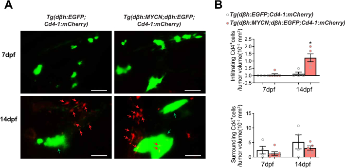
Figura 2. Mayor asociación de células CD4+ con lesiones de neuroblastoma que expresan MYCN a los 14 días post-fecundación. (A) Imágenes confocales representativas de peces control Tg(dβh:EGFP;Cd4-1:mCherry) y peces Tg(dβh:MYCN;dβh:EGFP;Cd4-1:mCherry) a los 7 y 14 días post-fecundación (dpf). Las células positivas para EGFP (verde) marcan células derivadas de la cresta neural/neuroblastoma que expresan dβh, y las células CD4+ están marcadas con mCherry (rojo). Las flechas indican células CD4+ representativas asociadas con la región de la cresta neural/tumor. Barras de escala = 50 µm. (B) Cuantificación de células CD4+ que rodean (abajo) e infiltran (arriba) la región de la cresta neural/tumor en peces control y en peces que expresan MYCN a los 7 y 14 dpf. Los conteos celulares se normalizaron respecto al volumen tumoral (células/mm3). Los datos se presentan como media ± EE. Las comparaciones estadísticas se realizaron mediante pruebas t no pareadas de dos colas. P < 0,05. n = 4 y 6 a los 7 dpf, y n = 4 y 5 a los 14 dpf para los grupos control y MYCN, respectivamente. Datos representativos de tres experimentos independientes. Haga clic aquí para ver una versión ampliada de esta figura.
Para examinar la asociación de células CD4+ con tumores establecidos, se criaron peces transgénicos compuestos clasificados hasta la edad adulta y se analizaron tras fijación, seccionamiento por criomicrotomía e imagen confocal (Figura 1). Se muestran imágenes representativas de neuroblastoma localizado y metastásico de peces de cuatro meses de edad en la Figura 3A. Los tumores se clasificaron como metastásicos cuando se detectaron células tumorales positivas para EGFP fuera de los ganglios simpáticos periféricos. Aplicamos un método de cuantificación basado en el área porque la microscopía confocal no puede capturar todo el volumen tumoral. Nuestro análisis reveló un número significativamente mayor de células CD4+ que rodeaban o infiltraban tumores metastásicos en comparación con tumores localizados (Figura 3B; P < 0,05; n = 4 por grupo). Los datos se presentan como recuentos celulares normalizados por área tumoral (células/mm2) y se expresan como media ± EE.
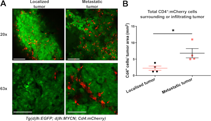
Figura 3. El neuroblastoma metastásico muestra una mayor infiltración de células CD4+ dentro del microambiente tumoral. (A) Imágenes confocales representativas de neuroblastoma localizado y metastásico desarrollado en peces cebra hermanos de 4 meses de edad Tg(dβh:MYCN;dβh:EGFP;Cd4-1:mCherry). Las células tumorales están marcadas con EGFP (verde) y las células CD4+ con mCherry (rojo). Las flechas indican células CD4+ representativas asociadas con el tejido tumoral. Se muestran imágenes adquiridas con objetivos de 20× y 63× como campos independientes de visión. Barras de escala = 100 µm (20×) y 50 µm (63×). (B) Cuantificación del número total de células CD4+ que rodean o infiltran tumores localizados y metastásicos. Los conteos celulares se normalizaron respecto al tamaño del tumor según se describe en el protocolo. Los datos se presentan como media ± EE. Las comparaciones estadísticas se realizaron mediante pruebas t no pareadas de dos colas. P < 0,05. n = 4 por grupo. Datos representativos de tres experimentos independientes. Haga clic aquí para ver una versión ampliada de esta figura.
Estos hallazgos demuestran que el protocolo puede utilizarse para visualizar y cuantificar células CD4+ asociadas con lesiones de neuroblastoma en múltiples etapas del desarrollo tumoral en pez cebra.
Vídeo suplementario 1. Serie z confocal representativa de un pez cebra control a los 7 días post-fecundación. Imagen tridimensional confocal de un pez cebra control Tg(dβh:EGFP;Cd4-1:mCherry) a los 7 días post-fecundación (dpf). Las células derivadas de la cresta neural positivas para EGFP se muestran en verde, y las células CD4+ se muestran en rojo. Pocas células CD4+ se observan dentro o alrededor de la región que expresa dβh en esta etapa del desarrollo. Haga clic aquí para descargar este archivo.
Vídeo suplementario 2. Serie z confocal representativa de un pez cebra que expresa MYCN a los 7 días post-fecundación. Imagen confocal tridimensional de un pez cebra Tg(dβh:MYCN;dβh:EGFP;Cd4-1:mCherry) a los 7 días post-fecundación (dpf). Las células premalignas de neuroblastoma que expresan MYCN positivas para EGFP se muestran en verde, y las células CD4+ se muestran en rojo. Similar a los peces control, se observan pocas celdas CD4+ dentro o alrededor de la región tumoral en esta etapa temprana del desarrollo. Haga clic aquí para descargar este archivo.
Vídeo suplementario 3. Serie de cortes z confocal representativa de un pez cebra control a los 14 días post-fecundación. Imagen tridimensional confocal de un pez cebra control Tg(dβh:EGFP;Cd4-1:mCherry) a los 14 días post-fecundación (dpf). Las células derivadas de la cresta neural positivas para EGFP aparecen en verde, y las células CD4+ aparecen en rojo. Las células CD4+ están distribuidas de forma dispersa y muestran una asociación limitada con la región que expresa dβh. Haga clic aquí para descargar este archivo.
Video suplementario 4. Serie z confocal representativa de un pez cebra que expresa MYCN a los 14 días post-fecundación. Imagen confocal tridimensional de un pez cebra Tg(dβh:MYCN;dβh:EGFP;Cd4-1:mCherry) a los 14 días post-fecundación (dpf). Las células premalignas de neuroblastoma que expresan MYCN positivas para EGFP se muestran en verde, y las células CD4+ se muestran en rojo. Se observa una acumulación e infiltración aumentada de células CD4+ en asociación con la región tumoral agrandada en comparación con peces control de edad coincidente, lo cual es consistente con la cuantificación mostrada en la Figura 2B. Haga clic aquí para descargar este archivo.
Discusión
El protocolo descrito aquí utiliza el pez cebra como un modelo in vivo para visualizar y cuantificar células inmunitarias dentro del microentorno tumoral (TME). Varios factores son fundamentales para la implementación exitosa de este enfoque. Primero, la selección y validación adecuadas de líneas transgénicas compuestas de pez cebra son esenciales. Las larvas deben examinarse para verificar los patrones esperados de expresión fluorescente y, si es necesario, confirmarse mediante genotipificación. Debe verificarse la expresión del reportero inmunitario y del oncogén antes del experimento para asegurar una asignación precisa de los grupos experimentales y de control. Segundo, la identificación precisa de la región de interés es fundamental durante la imagen confocal. La imagen en campo claro puede utilizarse para identificar puntos de referencia anatómicos y facilitar la localización del tejido objetivo. Por ejemplo, al imaginar tumores en la región anterior del cuerpo, el ojo puede usarse como punto de referencia para ayudar en la localización. Tercero, una colocación adecuada del pez es esencial para garantizar una exposición suficiente de la región de imagen. Una alineación inadecuada puede reducir la calidad de la imagen o dificultar la visualización del tejido de interés. Finalmente, es necesario un montaje e inmovilización adecuados para minimizar los artefactos por movimiento durante la imagen en vivo. La concentración de tricaina y la duración de la imagen deben optimizarse para mantener la viabilidad de las larvas preservando al mismo tiempo la calidad de la imagen.
La fototoxicidad puede minimizarse reduciendo la intensidad del láser y el tiempo de exposición durante la imagen en vivo. Para muestras adultas, los tejidos deben mantenerse sobre hielo durante el manejo y la preparación para la imagen, ya que los descongelamientos repetidos pueden alterar la integridad del tejido. El manejo cuidadoso de las muestras es particularmente importante tras la criocorte y la extracción del bloque de OCT.
La interpretación de los resultados de imágenes requiere considerar la especificidad del reportero. Varias líneas de reporteros inmunitarios etiquetan múltiples poblaciones de células inmunitarias. Por ejemplo, se ha reportado la expresión de CD4 en poblaciones celulares más allá de los linfocitos T convencionales, incluidos los macrófagos28. Además, además de los macrófagos, la expresión de mpeg también se detecta en células B29. Lysc puede etiquetar tanto neutrófilos como macrófagos30. Por consiguiente, la expresión fluorescente del reportero por sí sola puede no ser suficiente para asignar definitivamente la identidad celular. Enfoques adicionales de validación, como RNAscope, citometría de flujo, reacción en cadena de la polimerasa de transcripción inversa cuantitativa o secuenciación de ARN a nivel de célula individual, pueden complementar las observaciones basadas en imágenes y proporcionar una caracterización molecular adicional de las poblaciones celulares marcadas.
Este método tiene varias limitaciones. El enfoque depende de la expresión de un reportero fluorescente y, por lo tanto, no puede confirmar de forma independiente la identidad ni el estado funcional de las células inmunitarias. Además, el análisis de imágenes en el flujo de trabajo actual para peces adultos se basa en conjuntos de datos confocales proyectados de capas limitadas y puede no captar completamente las complejas relaciones celulares tridimensionales dentro del microentorno tumoral (TME). Por último, el método también requiere la generación y el mantenimiento de líneas de pez cebra transgénicas compuestas, lo que podría limitar su accesibilidad para algunos laboratorios.
A pesar de estas limitaciones, el protocolo proporciona un enfoque práctico para visualizar las células inmunitarias asociadas con lesiones de neuroblastoma en pez cebra. En comparación con la histología convencional de punto final, el método preserva la arquitectura tisular y permite la obtención de imágenes de células marcadas con fluorescencia dentro de tejidos intactos20,21. El flujo de trabajo puede aplicarse en múltiples etapas del desarrollo y puede adaptarse a otras líneas de reporteros fluorescentes. Además del neuroblastoma, múltiples estudios han realizado imágenes del microentorno tumoral (TME) para analizar la interacción entre melanoma y células inmunitarias, incluyendo células CD4+, macrófagos y células CD8+15,21,31,32. En conjunto, estas características convierten al protocolo en una plataforma útil para estudiar la localización de células inmunitarias dentro del TME del pez cebra.
Divulgaciones
Los autores declaran que no tienen intereses en competencia.
Agradecimientos
Agradecemos el apoyo de los National Institutes of Health (NIH; 1UL1TR001430, CA21059 y NS140967), la American Cancer Society (RSG-17-204-01-TBG), la National Science Foundation (1911253) y la Alex’s Lemonade Stand Foundation para H.F.; así como de una beca Warren Alpert Distinguished Scholars para X.Q. Y.W. recibió apoyo del Programa de Oportunidades de Investigación para Pregrado de la Universidad de Boston (UROP) y del Programa de Becas de Verano de St. Baldrick’s. M.V. recibió apoyo del Programa de Becas de Verano de St. Baldrick’s. El contenido de este artículo es únicamente responsabilidad de los autores y no representa necesariamente las opiniones oficiales de los NIH.
Materiales
| Nombre | Empresa | Número de catálogo | Comentarios |
|---|---|---|---|
| 200 µL de punta de carga para geles | MilliporeSigma | 1022-0600 | Utilizado para la manipulación de larvas |
| Plantas artificiales | The Hidden Reef | 62874200000000000 | Enriquecimiento opcional para reproducción |
| Lejía | Fisher Scientific | 50371500 | Utilizada para la descontaminación de embriones |
| Complemento para contador de células | National Institutes of Health (NIH) | N/A | Complemento de Fiji utilizado para la cuantificación celular |
| Computadora y monitor | HP | 2TB68A8#ABA | Utilizado para la adquisición y análisis de imágenes |
| Microscopio confocal | Zeiss | LSM 710 | Utilizado para imágenes de larvas y adultos |
| Molde criogénico, plástico | Epredia | 22-050-160 | Utilizado para inclusión en OCT |
| Criostato | Thermo Fisher Scientific | 95-664-0EC70 | Utilizado para corte criogénico |
| Hielo seco | Fisher Scientific | N/A | Utilizado para el transporte de muestras |
| Software Fiji | National Institutes of Health (NIH) | Version 1.54p | Software para análisis de imágenes |
| Red de malla fina | Carolina Biological | 651345 | Utilizada para la recolección de embriones |
| Incubadora para peces | VWR | 35960-056 | Mantenida a 28.5°C |
| Pinzas | Fisher Scientific | 10-316B | Utilizadas para el manejo de muestras |
| Placa de fondo de vidrio | IBIDI | 81218-200 | Utilizada para imágenes |
| Agarosa de bajo punto de fusión | Prolab Supply | 9012-36-6 | Utilizada para montaje de larvas y adultos |
| Tanque de apareamiento (tanque principal, divisor, sección con rejilla) | Carolina Biological | 161937 | Utilizado para la reproducción de pez cebra |
| Agitador rotatorio | Midsci | R2D-30 | Utilizado para fijación durante incubación nocturna |
| Compuesto OCT | Tissue-Tek | 4583 | Medio de inclusión para corte criogénico |
| Paraformaldehído (PFA) | Sigma Aldrich | 158127-500G | Fijador |
| Placa de Petri, plástica | MilliporeSigma | BR452000 | Utilizada para el manejo de embriones y larvas |
| Solución salina tamponada con fosfato (PBS) | Gibco | 14080-055 | Utilizada para lavados y procedimientos de fijación |
| Pipeta de transferencia plástica | Fisher Scientific | 50-998-100 | Utilizada para la transferencia de embriones y larvas |
| Cuchilla de afeitar | Fisher Scientific | 12-640 | Utilizada durante la preparación de muestras |
| Medidor de conductividad | YSI | EC300ACC-04 | Utilizado para verificar la salinidad del agua de rotíferos |
| Rotíferos | The Hidden Reef | 116151603 | Utilizados para el cultivo de larvas |
| Tiosulfato de sodio | Thermo Fisher Scientific | AAA1762936 | Utilizado para la neutralización de lejía |
| Sacarosa | Fisher Scientific | S25590A | Reactivo de crioprotección |
| Tricaina metanosulfonato | Western Chemical | NC0872873 | Anestésico; vendido por Fisher Scientific |
| Tenazas | Fisher Scientific | 12-000-122 | Utilizadas para el manejo de muestras |
| Microscopio de fluorescencia invertido | Leica | M165 | Utilizado para cribado de fluorescencia |
Referencias
- Anderson NM, Simon MC. The tumor microenvironment. Curr Biol. 2020;30(16):R921-R925.
- Kumagai S, Momoi Y, Nishikawa H. Immunogenomic cancer evolution: A framework to understand cancer immunosuppression. Sci Immunol. 2025;10(105):eabo5570.
- Keren L, et al. A structured tumor-immune microenvironment in triple negative breast cancer revealed by multiplexed ion beam imaging. Cell. 2018;174(6):1373-1387.e19.
- Gerner MY, et al. Histo-cytometry: A method for highly multiplex quantitative tissue imaging analysis applied to dendritic cell subset microanatomy in lymph nodes. Immunity. 2012;37(2):364-376.
- Pittet MJ, Weissleder R. Intravital imaging. Cell. 2011;147(5):983-991.
- Wienke J, et al. The immune landscape of neuroblastoma: Challenges and opportunities for novel therapeutic strategies in pediatric oncology. Eur J Cancer. 2021;144:123-150.
- Spitzer MH, Nolan GP. Mass cytometry: Single cells, many features. Cell. 2016;165(4):780-791.
- Roy D, et al. Zebrafish—A suitable model for rapid translation of effective therapies for pediatric cancers. Cancers (Basel). 2024;16(7):1361.
- White RM, et al. Transparent adult zebrafish as a tool for in vivo transplantation analysis. Cell Stem Cell. 2008;2(2):183-189.
- MacRae CA, Peterson RT. Zebrafish as tools for drug discovery. Nat Rev Drug Discov. 2015;14(10):721-731.
- Miao KZ, et al. Tipping the scales with zebrafish to understand adaptive tumor immunity. Front Cell Dev Biol. 2021;9:660969.
- Povoa V, et al. Innate immune evasion revealed in a colorectal zebrafish xenograft model. Nat Commun. 2021;12(1):1156.
- Wang J, et al. Novel mechanism of macrophage-mediated metastasis revealed in a zebrafish model of tumor development. Cancer Res. 2015;75(2):306-315.
- Loveless R, Shay C, Teng Y. Unveiling tumor microenvironment interactions using zebrafish models. Front Mol Biosci. 2020;7:611847.
- Dee CT, et al. CD4-transgenic zebrafish reveal tissue-resident Th2- and regulatory T cell-like populations and diverse mononuclear phagocytes. J Immunol. 2016;197(9):3520-3530.
- Murali Shankar N, et al. Preclinical assessment of CAR-NK cell-mediated killing efficacy and pharmacokinetics in a rapid zebrafish xenograft model of metastatic breast cancer. Front Immunol. 2023;14:1254821.
- Tan KE, et al. LMO1 expression in neuroblastoma cells reprograms tumor-associated macrophages to promote metastasis. iScience. 2026;29(3):115144.
- Fior R, et al. Single-cell functional and chemosensitive profiling of combinatorial colorectal therapy in zebrafish xenografts. Proc Natl Acad Sci U S A. 2017;114(39):E8234-E8243.
- Fazio M, et al. Zebrafish patient avatars in cancer biology and precision cancer therapy. Nat Rev Cancer. 2020;20(5):263-273.
- Qin X, et al. CKLF instigates a “cold” microenvironment to promote MYCN-mediated tumor aggressiveness. Sci Adv. 2024;10(11):eadh9547.
- Ludin A, et al. CRATER tumor niches facilitate CD8+ T cell engagement and correspond with immunotherapy success. Cell. 2025;188(24):6720-6736.e26.
- Zhu S, et al. LMO1 synergizes with MYCN to promote neuroblastoma initiation and metastasis. Cancer Cell. 2017;32(3):310-323.e5.
- Tao T, et al. The pre-rRNA processing factor DEF is rate limiting for the pathogenesis of MYCN-driven neuroblastoma. Oncogene. 2017;36(27):3852-3867.
- Zimmerman MW, et al. MYC drives a subset of high-risk pediatric neuroblastomas and is activated through mechanisms including enhancer hijacking and focal enhancer amplification. Cancer Discov. 2018;8(3):320-335.
- Dankert EN, Look AT, Zhu S. Unraveling neuroblastoma pathogenesis with the zebrafish. Cell Cycle. 2018;17(4):395-396.
- Langenau DM, et al. In vivo tracking of T cell development, ablation, and engraftment in transgenic zebrafish. Proc Natl Acad Sci U S A. 2004;101(19):7369-7374.
- Lam SH, et al. Development and maturation of the immune system in zebrafish, Danio rerio: A gene expression profiling, in situ hybridization and immunological study. Dev Comp Immunol. 2004;28(1):9-28.
- Zhen A, et al. CD4 ligation on human blood monocytes triggers macrophage differentiation and enhances HIV infection. J Virol. 2014;88(17):9934-9946.
- Ferrero G, et al. The macrophage-expressed gene (mpeg)1 identifies a subpopulation of B cells in the adult zebrafish. J Leukoc Biol. 2020;107(3):431-443.
- Hall C, et al. The zebrafish lysozyme C promoter drives myeloid-specific expression in transgenic fish. BMC Dev Biol. 2007;7:42.
- Lorenzini F, et al. Melanoma innervation, noradrenaline and cancer progression in zebrafish xenograft model. Cell Death Discov. 2025;11(1):260.
- Ramakrishnan G, et al. Real-time imaging reveals a role for macrophage protrusive motility in melanoma invasion. J Cell Biol. 2025;224(2):e202403096.
Reimpresiones y permisos
Este artículo ha sido publicado
Video próximamente