Analysis of Tubular Membrane Networks in Cardiac Myocytes from Atria and Ventricles

Summary

In cardiac myocytes, tubular membrane structures form intracellular networks. We describe optimized protocols for i) isolation of myocytes from mouse heart including quality control, ii) live cell staining for state-of-the-art fluorescence microscopy, and iii) direct image analysis to quantify the component complexity and the plasticity of intracellular membrane networks.

Abstract

In cardiac myocytes a complex network of membrane tubules - the transverse-axial tubule system (TATS) - controls deep intracellular signaling functions. While the outer surface membrane and associated TATS membrane components appear to be continuous, there are substantial differences in lipid and protein content. In ventricular myocytes (VMs), certain TATS components are highly abundant contributing to rectilinear tubule networks and regular branching 3D architectures. It is thought that peripheral TATS components propagate action potentials from the cell surface to thousands of remote intracellular sarcoendoplasmic reticulum (SER) membrane contact domains, thereby activating intracellular Ca²⁺ release units (CRUs). In contrast to VMs, the organization and functional role of TATS membranes in atrial myocytes (AMs) is significantly different and much less understood. Taken together, quantitative structural characterization of TATS membrane networks in healthy and diseased myocytes is an essential prerequisite towards better understanding of functional plasticity and pathophysiological reorganization. Here, we present a strategic combination of protocols for direct quantitative analysis of TATS membrane networks in living VMs and AMs. For this, we accompany primary cell isolations of mouse VMs and/or AMs with critical quality control steps and direct membrane staining protocols for fluorescence imaging of TATS membranes. Using an optimized workflow for confocal or superresolution TATS image processing, binarized and skeletonized data are generated for quantitative analysis of the TATS network and its components. Unlike previously published indirect regional aggregate image analysis strategies, our protocols enable direct characterization of specific components and derive complex physiological properties of TATS membrane networks in living myocytes with high throughput and open access software tools. In summary, the combined protocol strategy can be readily applied for quantitative TATS network studies during physiological myocyte adaptation or disease changes, comparison of different cardiac or skeletal muscle cell types, phenotyping of transgenic models, and pharmacological or therapeutic interventions.

Introduction

In healthy striated muscle cells, tubular membrane structures with “transverse” orientations (T-tubules) perpendicular to the main cell axis are abundant. Consequently, T-tubules have been characterized as continuous extensions of the muscle cell main “lateral” surface membrane (sarcolemma), which deeply penetrate the cytosol towards the cell center. The physiological role of T-tubules continuous with the outer surface membrane is the rapid electrical coupling of remote intracellular compartments formed by SER organelle contact domains throughout the relatively large cardiac muscle cell volume by nanometric proximity coupling of voltage-activated L-type Ca²⁺ channels (Cav1.2) inward current (I_Ca) activating adjacent ryanodine receptor (RyR2) SER Ca²⁺ releases. In ventricular myocytes (VMs), the non-continuous membrane contacts (“junctions”) between the junctional SER domains and T-tubules are thought to control thousands of individual intracellular Ca²⁺ release nanodomains in each cell¹.

For any given contact domain, the juxtaposed membrane portions each of the T-tubule and the peripheral (junctional) SER are approximately 15 nm close to each other, hence defined as nanodomain. Thereby, very small individual cytoplasmic subspaces are segregated which enable quasi cell-autonomous compartment behaviors. When an incoming action potential activates Cav1.2 channels in the T-tubules of VMs, a relatively small Ca²⁺ inward current will rapidly increase the subspace Ca²⁺ concentration [Ca²⁺]_S in the attoliter sized nanodomain¹. Next, the [Ca²⁺]_S increase activates Ca²⁺-gated ryanodine receptors (RyR2) within nanometer proximity in the juxtaposed SER membrane junction, and this coupling process occurs throughout all electrically coupled myocyte nanodomains. RyR2s occur as dense multi-channel clusters with an estimated stoichiometry of 1 Cav1.2 channel for 5-10 RyR2 channels². Since the SER-to-cytosol [Ca²⁺] gradient is very steep (ratio 10⁴:1) and RyR2s function as high-conductance Ca²⁺ release channels in functionally coupled clusters, RyR2 activation results in a quantitatively large Ca²⁺ release current from T-tubule coupled junctional SER domains increasing local subspace [Ca²⁺]_S to 100 µM or higher within 1-2 msec^3,4. This cardiac signal amplification behavior is also referred to as Ca²⁺ induced Ca²⁺ release (CICR). Taken together, T-tubules are essential membrane structures that rapidly activate Ca²⁺ release signals through junctional nanodomain SER contacts and cell-wide CICR during excitation-contraction (EC) coupling.

In addition to T-tubules, axial tubules (A-tubules) with a significantly different orientation parallel to the main (longitudinal) cell axis have been documented by electron microscopy (EM), confocal and 2-photon microscopy studies. For instance, a cell-wide continuous lattice of A-tubules between myofibrils interconnected with T-tubules near sarcomere Z-lines was shown by extracellular tracers and EM imaging of fixed guinea pig VMs⁵. Using extracellular dextran-linked fluorescein staining and live 2-photon imaging of rat VMs, a complex reticular 3D tubule network was visualized consisting of ~60% T-tubules and ~40% A-tubules⁶. This study not only led to 3D visualization of abundant A-tubules, but also to the realization that sectioning for EM visualization is inherently limited for the analysis of complex and dynamic membrane networks like the transverse-axial tubule system (TATS). Consequently, confocal live cell imaging of TATS membranes directly stained with di-8-ANNEPS was developed. If live cell TATS networks are analyzed by Fourier transformation, the regular appearance of T-tubule components in space near sarcomere Z-lines is reflected by the ensemble power spectrum from a region of striated signals⁷. This indirect analysis strategy has been used to detect cell-wide regional changes in TATS component regularity in disease models⁷. For instance, shRNA mediated junctophilin-2 knock-down caused heart failure and the isoform specific protein deficiency resulted in T-tubule reorganization with nanodomain Ca²⁺ release dysfunction⁸. We have recently extended the analysis of TATS membrane networks through direct quantitative approaches and further by live cell superresolution microscopy of individual TATS components in mouse VMs using stimulated emission depletion (STED) nanoscopy⁹. Nanometric image resolution allowed for direct analysis of smaller individual TATS components, which approximate a 50:50 distribution of transverse versus axial tubule orientations, quantitatively confirming two abundant yet differentially oriented individual TATS components in healthy mouse hearts⁹. These strategies will be further outlined in the protocol section below.

While the physiological role of the abundant A-tubule components in the adult heart has remained enigmatic, EM studies have documented SER membrane structures associated with A-tubules suggesting endogenous Ca²⁺ release nanodomains in guinea pig and rat VMs^5,10. Confocal analysis of Cav1.2 and RyR2 found a high degree of colocalization at A-tubule junctions¹⁰. Since ~20% of spontaneous Ca²⁺ sparks in rat VMs originated relatively far away from Z-line striations where T-tubules typically occur, one argument has been that A-tubule associated nanodomains may indeed exist and function as Ca²⁺ release sites^11,12. Interestingly, T-tubule formation and maturation occurs only after birth and parallels the growth of cardiac cells, e.g., through sprouting of precursor sarcolemmal invaginations at P5 and immature branched TATS network assemblies at P10 in mice¹³. It appears that Junctophilin-2 is particularly important for postnatal TATS network maturation since shRNA knock-down prevented the anchoring of T-tubule membranes to SER junctions leading to delayed Ca²⁺ release and pathological TATS organization consistent with immature A-tubule dominated architectures in VMs¹³. These observations may ultimately lead to proof-of-concept that T-tubules form through membrane invagination processes whereas A-tubules may morph through additional or even alternative intracellular mechanisms¹⁴.

Characterization of TATS membrane changes in heart disease has become an important research area for pathophysiological questions. Initial reports in a dog model of pacing-induced heart failure showed a loss of T-tubules and Cav1.2 current (I_Ca)¹⁵. A pig model of ischemic cardiomyopathy showed reduced T-tubule densities and a reduced synchrony of intracellular Ca²⁺ release¹⁶. Using a spontaneously hypertensive rat (SHR) model of heart failure, a loss of T-tubules was associated with reduced nanodomain coupling of Cav1.2 and RyR2 by the proposed mechanism of “RyR2 orphaning”⁷. A loss of T-tubules has also been shown in human VMs from ischemic, dilated, and hypertrophic cardiomyopathy samples¹⁷. Furthermore, an increase in A-tubules was reported in tissue sections of human dilated cardiomyopathy¹⁸. Following myocardial infarction, we showed a differential mechanism of TATS reorganization in mouse VMs with significant decreases of T-tubules in contrast to increases of A-tubule components⁹. Importantly, improved local membrane contrast achieved through live cell superresolution STED microscopy enabled detailed quantitative component analysis through direct measurements, which showed significant proliferation of the A-tubules with overall increases of the TATS network length and branching complexity⁹. Moreover, it was shown that exercise training may reverse T-tubule remodeling in rats after myocardial infarction¹⁹ and that cardiac resynchronization therapy may lead to reverse remodeling of T-tubules in dogs with atrial tachypacing induced heart failure²⁰. Taken together, studies both in diseased human and animal VMs as well as potential therapeutic interventions will arguably benefit from high quality cell isolation procedures and detailed quantitative analysis strategies as outlined in the protocol and results sections below.

Furthermore, as demonstrated recently by lateral surface versus TATS membrane trafficking of KATP channel isoforms ²¹, it is important to consider atrial myocytes (AMs) as biologically distinct as well as comparative cardiac cell model versus VMs. T-tubules were recently documented in sheep and human AMs²². Current evidence suggests that few T-tubules exist in AM cells and typically in larger mammals like sheep and humans, but not in small rodents²³. In contrast to VMs, in AMs intracellular Ca²⁺ release appears to occur from the cell surface propagating by diffusion towards the cell center which results in marked spatial and temporal Ca²⁺ gradients²³. Within this framework it seems important to elucidate mechanisms of intracellular Ca²⁺ signaling instability for common disease forms such as atrial fibrillation²⁴. In summary, both AM and VM cell isolation and each for healthy and diseased hearts are commonly employed protocols. Only if cell isolation is done properly as judged by microscopic documentation of sufficient cell quality, AM and VM samples should be carried forward for quantitative TATS analysis. Accordingly, the following protocol sections are critically dependent on high quality cell isolates from mouse or other species followed by live cell microscopy to analyze intact TATS membranes. As pointed out previously, characterization of TATS membranes is a challenging research area with a propensity for fixation and preparation artifacts⁶, membrane changes due to osmotic alterations, and resolution limitations of conventional light microscopy⁹. We note that recent state-of-the-art protocols for isolation of human AMs for Ca²⁺ imaging and patch-clamp and of rat VMs for cell culture have been previously published in this journal^25,26.

Protocol

NOTE: All animal procedures were reviewed and approved by the Institutional Animal Care and Use Committee of the University Medical Center Goettingen in compliance with the humane care and use of laboratory animals.

1. Isolation of Atrial and Ventricular Myocytes from the Mouse Heart

1. Handle animals as gently as possible and according to approved protocols to minimize stress in general and specifically to avoid potential powerful inadvertent effects from neurohormonal excesses on isolated cardiac cells. In addition, inject each mouse with heparin (500 IU/kg body weight s.c.) at least 20 min prior to heart extraction to prevent blood clotting and micro emboli which can significantly compromise the yield and integrity of cardiac cells during isolation.
2. Anesthetize mice aged 12 weeks or older by isoflurane inhalation, confirm absence of pain withdrawal reflexes, and euthanize animals by cervical dislocation.
   1. Extract the heart swiftly following previously established expert protocols (e.g., see Kaestner et al.²⁶ and Louch et al.²⁷). Avoid any inadvertent damage to the atria by unnecessary squeezing or stretching.
   2. Carefully preserve the tissue of the proximal ascending aorta using a pair of stump forceps and straight scissors to establish a continuous transversal cutting edge through the aortic vessel wall, which is important for successful cannulation and perfusion of the heart.
3. Transfer the excised heart immediately into ice-cold nominally Ca²⁺ free perfusion buffer (for solutions see Table 1). Keep the great vessels clamped during transfer through air into buffer to avoid inadvertent air embolism until the heart is fully submerged. Use BDM in the buffer and ice-cooled solutions to inhibit cardiac contraction.
4. Use a binocular zoom microscope with sufficient 3D illumination.
   1. Cannulate the aorta under panoramic stereovision of the heart with a smooth, surface polished 21 G cannula (outer diameter 0.81 mm; for normal mouse heart weight) which must be completely filled with buffer. Ensure that there are no air bubbles in the cannula by connecting a proximal solution reservoir (e.g., a syringe) through a 2-way Luer valve allowing for rapid solution flow control.
   2. Confirm under binocular magnification that the cannula is positioned correctly inside the aorta, which is approximately 1 mm above the aortic valves and coronary artery branches. Absolutely avoid any passage through or inadvertent perforation of the aortic valves with the cannula (this will permanently disrupt aortic valve closure and consequently disrupt cardiac perfusion).
5. Tie the aorta gently to custom-made, circumferentially oriented anti-slip grooves near the end of the cannula using two silk sutures. Do not flush the coronary arteries forcefully at any point. Connect the solution filled cannula tied to the aorta and the heart to a tightly fitting outflow connector of a customized and pre-calibrated perfusion system, a.k.a. the modified Langendorff setup (either using constant pressure or constant flow; see also discussion section below).
6. Perfuse the heart as soon as possible for 4 min using oxygenated perfusion buffer at 37 °C (target perfusion rate: 4 ml/min). Start the digestion by switching the perfusion to collagenase containing digestion buffer (600 U/ml collagenase type II) for 8-10 min at 37 °C. Monitor the progress of tissue digestion by confirming similar tissue changes including increasing opaqueness, softness, and flaccidity throughout the apparent heart surface.
7. Dissect the cardiac chambers as needed following digestion. Place the cannulated heart under a binocular microscope and visualize the posterior heart wall. Dissect residual non-cardiac tissue e.g., lung and vessel parts to avoid cell contamination in the digestion buffer using micro scissors (e.g., spring scissors with 8 mm straight blades) as shown in Figure 1.
8. Follow a check list which particular chambers, regions, and/or cells of the collagenase digested heart should be harvested (Figure 1): left and/or right atrium, free left and/or right ventricular wall, and/or the ventricular septum.
   1. For dissection of specific cardiac tissues, use a relatively wide and flat dissection bath coated with a several mm thick layer of silicone plastic elastomer. Fix the apex of the heart with a fine insect steel pin to the bottom elastomer layer.
   2. Deflect the right atrial appendage and dissect the right atrium just above the atrioventricular valves. Continue the dissection with the left atrium. Dissect and discard the fibrous valve apparatus. Finally, dissect the left and right free ventricular walls and the septum and/or smaller tissue parts as needed.
   3. Note only for trainees: to gain practice, start with non-digested mouse hearts. For ease of anatomical orientation, practice the tissue handling including all consecutive dissection steps under binocular vision as shown in Figure 1. Once the 3D anatomy, manual handling under binocular vision, and dissection steps are sufficiently familiarized, continue with the collagenase digested mouse hearts as outlined above.
9. For ventricular myocyte (VM) cell isolation: transfer the ventricular tissue into 2.5 ml of fresh digestion buffer. If simultaneous cell isolations from several organ parts, e.g., atria and ventricles is attempted, a second person may take over one leg of the cell dissociation procedure, both to minimize and optimize use of mice through coordinated handling of multiple cardiac tissues. Continue with steps 1.9.1-1.9.4, thereafter 1.10.
   1. Dissect either the entire ventricular tissue or specific parts thereof (e.g., LV, RV, free walls, and/or septum) into approximately 1 mm³ pieces in 2.5 ml digestion buffer using sharp scissors (e.g., spring scissors with 8 mm straight blades) in a 60 mm Petri dish.
   2. Gently dissociate VMs into cell suspension by slow trituration of the tissue pieces with a transfer pipette. Avoid any air bubbling in cell suspension.
   3. Add 8 ml of stop buffer to the VM cell suspension and transfer the cell suspension into a 15 ml conical tube. Allow the remaining tissue pieces to settle at the bottom for approximately 15 sec, but short enough for isolated cells to remain in suspension. Next, harvest the VM suspension via transfer of the supernatant volume to a new 15 ml tube. If excessive tissue pieces are present, alternatively use a minimally 200 µm spaced nylon mesh to separate the tissue pieces from the cell suspension.
   4. Let the VM cell suspension settle to the bottom of a 15 ml conical tube by gravity for 8 min.
   5. Wash step: remove the supernatant and gently resuspend the remaining VM pellet in 10 ml of perfusion buffer. Repeat wash step 1.9.5 (optional: add additional wash steps to gradually increase the Ca²⁺ concentration as needed).
   6. Resuspend the settled VM pellet in 10 ml perfusion buffer and distribute the remaining cell suspension volume in 1.5 ml microcentrifuge tubes (approximately 50,000 VM cells per tube).
10. For atrial myocyte (AM) cell isolation: transfer the digested/dissected atrial tissue into 1 ml of fresh digestion buffer.
    1. Cut the partially digested atrial tissue into approximately 1 mm³ pieces in 1 ml digestion buffer using micro scissors in a small Petri dish (e.g., 60 mm diameter). Gently dissociate AM cells out of the digested tissue pieces into cell suspension using trituration with a 1 ml plastic pipette with a cut tip to avoid damaging fluid jets. During trituration strictly avoid any air bubbling in cell suspension. Following mechanical agitation, add 4 ml of stop buffer (50 µM CaCl₂; 10% BCS) to arrest any remaining collagenase activity in cell suspension.
    2. Transfer the AM cell suspension into a 15 ml conical tube. Allow the remaining tissue pieces to settle at the bottom for approximately 15 sec, but short enough for the isolated cells to remain in suspension. Harvest the supernatant volume containing the free AM cells via solution transfer to a new 15 ml tube.
    3. Centrifuge the AM cell suspension, e.g., 2 min at 20 x g at RT or - preferable for membrane studies - let the cells settle down slowly by gravity for 20 min in a 15 ml conical tube.
    4. Wash step: discard the supernatant and gently resuspend the AM pellet in 5 ml perfusion buffer. Repeat 1.10.4.
    5. Resuspend AM cells gently in 5 ml perfusion buffer. Distribute the cell suspension volume in 1.5 ml microcentrifuge tubes (approximately 1,000 AM cells per tube).
11. Analyze and document the isolated cell population quality for each heart including the cell yield using trypan blue staining.
    1. For this, dilute 500 µl of the cell suspension as 1:1 vol/vol with trypan blue solution (final concentration 0.02%) using 1 ml cut pipette tips. Mix the cells and the trypan blue gently by very slow up/down pipetting. Immediately apply the trypan blue containing cell suspension to a Neubauer-type improved cytometer and count the intact myocytes using an inverted microscope.
    2. Exclude any cells with apparent damage, membrane blebs, disrupted striations, contractures, and cells accumulating intracellular trypan blue (Figure 2). Also exclude spontaneously contracting cells, which are susceptible to subsequent cell death. To assess the count of intact cells in suspension, use only cardiac myocytes with regular striations which exclude trypan blue throughout the cell volume.
12. Judge the integrity of individual atrial and ventricular myocytes by transmitted light microscopy. Save the bright field image as a Tif file for documentation and further analysis.
    1. Use the following criteria for analysis of cardiac cell integrity:
       1. confirm the presence of regular striations throughout the visible cell volume;
       2. confirm the continuous integrity of the lateral surface membrane on both cell sides parallel to the myofilaments;
       3. visualize sharp serrations at the intercalated discs on both cell sides which reflect the integrity of specific surface membrane structures; and
       4. visualize the fluorescent signals of TATS membranes (or immunolabeled caveolin-3 protein or other membrane markers) as described in section 3 for localization correlation next to the underlying cell-specific bright field image morphology (e.g., combine both images with ImageJ as overlay compound image).
       5. Determine the sarcomere length from the bright field images. For mean sarcomere length, measure the distance of sequentially aligned sarcomere striations, and divide the distance by the number of sarcomeres. Measure at least two locations per cell. Perform the analysis with commercial software or offline with ImageJ.
          NOTE: If treated with uncoupling agents, intact relaxed VMs from mouse heart show a mean sarcomere length of ~1.9 µm²⁸.
13. Quantify the morphology and dimensions of individual atrial and ventricular myocytes from the transmitted light microscopy image. Consider that AM and VM cells differ significantly in size. Measure the cell length, width, and area, and calculate the length:width ratio.
    1. Analyze the 2D cell dimensions from the transmitted light image in ImageJ using the commands polygon selection tool and add to ROI manager, analogous to Figure 3. If morphological changes are expected within specific study contexts, further document for all cells the specific mouse strain, age, sex, heart size, and any interventions for subsequent data classification.

2. Staining of TATS Membranes in Living Atrial and Ventricular Myocytes

1. Load the imaging chamber (e.g., POC-R2) with a 42 mm glass coverslip. For stable myocyte attachment to the coverslip, prepare 20 µl of laminin solution by 1:10 dilution of the laminin stock in physiological perfusion buffer (final concentration 0.2 mg/ml). Spread 20 µl of the laminin solution evenly on the glass coverslip.
2. Prepare 800 µl of a 50 µM di-8-ANEPPS solution in perfusion buffer. For this, dilute 20 µl of 2 mM di-8-ANEPPS stock solution in 780 µl physiological buffer.
3. To stain VMs, let the cells settle by gravity for 8 min in a 1.5 ml reaction tube. To stain AMs, either use gravity sedimentation or spin the cell suspension for 2 min (refer to 1.10.3). For both AMs and VMs, carefully remove the supernatant while avoiding unnecessary agitation of the cell pellet and gently resuspend the cell pellet in 800 µl of di-8-ANEPPS containing solution (50 µM). Immediately transfer the di-8-ANEPPS/myocyte suspension onto the laminin-coated coverslip in the imaging chamber.
4. Stain the VM suspension for 15 min at RT in the dark.
5. Slowly remove excess volume via the upward fluid meniscus at the sides of the imaging chamber with a manual pipette. Confirm that the majority of di-8-ANEPPS stained myocytes remains firmly attached to the laminin-coated coverslip and do not become exposed to air. Next, wash the attached myocyte suspension once by slowly adding 1 ml of perfusion buffer followed by removing any excess fluid including non-adherent cells.
6. Carefully overlay the stained and surface attached myocytes with 1 ml of perfusion buffer slowly from the side of the imaging chamber. Place the imaging chamber on the microscope stage.

3. Imaging of TATS Membrane Structures in Living Atrial and Ventricular Myocytes

1. In general, carefully choose the best possible fluorescent microscope option(s) available for TATS membrane imaging. For confocal imaging, consider recent generation, modern fluorescence microscopes with optimized PMT array detectors and photon recycling pathways that maximize fluorescent signal intensity. For confocal imaging of smaller details of TATS membrane structures use a 63X 1.4 NA oil objective or – depending on availability – use a STED superresolution microscope for smallest TATS details as reviewed for myocyte-specific applications by Kohl et al.³⁴ For general principles of high resolution fluorescence microscopy, refer to the discussion section.
2. Set the imaging parameters to detect most, ideally all di-8-ANEPPS stained intracellular membranes inside a given myocyte imaging plane. Use the following parameters as starting point for confocal laser scanning microscopy: excitation 458 nm e.g., at 3% of the maximal laser power; detect the emitted signal between 550 nm and 740 nm; detector gain (e.g., master command 800); and pinhole 1 AU for an optical slice thickness of 900 nm. Adjust these parameters to optimize the signal-to-noise.
3. Use the bright field mode to select an intact AM or VM cell as appropriate (Figures 4A and 4B). Refer to point 1.12 for relevant criteria how to judge cell integrity to select cells as summarized: cell-wide regular striations and equal sarcomere spacing, sharp surface edges and serrations on all four cell sides, continuous integrity of the lateral surface membrane, and absence of any membrane blebs.
4. Take a sample image of a central intracellular myocyte section. To adjust the ROI use the “crop” function →adjust the crop window →the final pixel size measures 100 nm x 100 nm. Adjust the x-axis of the crop window to correspond with the major (axial / longitudinal) axis of the myocyte.
5. Select the final imaging plane. Use single image frames to manually select the appropriate imaging plane in the z-direction. Confirm that the TATS membranes, including T-tubule and A-tubule components, are visually apparent in the focal plane. Note that a typical intracellular imaging plane may include a nucleus as intracellular reference point. Refer to the examples in Figures 4A and 4B.
   NOTE: In general, keep cell exposure to laser light as short as possible. If possible, use single image frames to determine the optimal focal plane in cardiac myocytes.
6. Adjust the pixel dwell time to approximately 0.5 µsec. Select 16x averaging and record the image as snapshot. Repeat the image snapshot step to establish the appropriate imaging plane as outlined for TATS membrane structures in 3.5 as needed.
7. Save the final image and confirm that the file was saved in its target folder. In general, save all image files in the same format (e.g., lsm) for uniform application of analysis software. Prior to any image analysis, once again confirm sufficient cell integrity off-line (consider criteria listed under step 1.12.1) and exclude any damaged cells from analysis. Refer to the examples in Figures 4C and 4D.

4. Analysis of the TATS Membrane Network and its Components

The following image processing steps for direct analysis of TATS membrane components are summarized as top-down workflow diagram in Figures 5A and 5B.

1. Open the image file of a di-8-ANEPPS stained myocyte in Fiji (http://fiji.sc/), a freely available variant of ImageJ which contains analysis plugins essential for image processing. For further information please refer to Schindelin et al²⁹.
2. Save the image →File →Save As →Tif.
3. To analyze the TATS membrane components, select the appropriate ROI excluding the outer surface membrane signal, then use the “polygon selection” tool to delineate the ROI border excluding the outer surface membrane (sarcolemma) and including the intracellular portions of TATS membranes as shown in Figure 5A (ROI). Add the selected ROI to the “ROI Manager” by applying Analyze →Tools →ROI Manager.
   1. To select a specific ROI for the orientation analysis of TATS components, align the main longitudinal cell axis and the image x-axis in parallel. If the cell is slightly curved, select several ROIs and align each ROI individually. Exclude any nuclei from the analysis. Exclude any excessively curved cells from the analysis because precise alignment of ROIs will become increasingly difficult and increase orientation errors during analysis.
4. Delete any unwanted signal information from the outer surface membrane: Edit →Clear Outside to generate the “selected ROI” (Figure 5A). Ensure that the selected ROI only contains the intracellular membrane portions, which correspond with the TATS network.
5. Perform the following chain of image processing steps (commands) prior to the subsequent quantitative analysis as documented in Figure 5A.
   1. Click on →Process →Subtract Background. Set the Rolling ball radius to 5 pixels.
      NOTE: Set the rolling ball radius to 5 pixels if the image to be analyzed has a pixel size of 100 nm x 100 nm. For other pixel sizes set the rolling ball radius to the number of pixels which approximately correspond to a physical radius of 500 nm.
   2. Click on →Process →Enhance Local Contrast (CLAHE). Set the block size to 49, the histogram bins to 256, the maximum slope to 3, and the mask to “none”.
   3. Click on →Process →Smooth.
   4. Click on →Plugins →Segmentation →Statistical Region Merging. Set the parameters to Q100 →click on Show Averages.
   5. Confirm complete processing of the statistical region merging indicated by automatic presentation of a new image frame and confirm that the label “SRM Q=100” appears. Continue the following steps with this image file. Click on →Image →Type →8-bit.
   6. Click on →Image →Adjust →Threshold. Choose the threshold sufficiently low to detect most, ideally all TATS structures, in particular avoid exclusion of TATS components with a low signal intensity (use a threshold of 40 as starting point). Consult the “Representative Results” section for detailed data output and the examples in Figure 6 (upper threshold of 255). Document the final choice of threshold parameters. Note that the correct choice of threshold should produce only specific TATS membrane structures but not false positive signals due to background noise.
   7. Confirm correct superimposition of TATS image details versus extracted skeleton data, in particular for intermediate and high fluorescence signal levels, which should match the (dis-) continuity of the skeleton structure. Once an appropriate threshold has been identified, apply this same threshold to all images during analysis and repeat the overlay comparison of the original signal versus skeleton data to consistently minimize this potential source of bias.
   8. Click on →Apply: the image data becomes binary as shown in Figure 5 under “Threshold”.
   9. Click on →Plugins →Skeleton →Skeletonize (2D/3D). Save the skeletonized 2D image (as shown in Figure 5) as Tif file by clicking on →File →Save as →Tif. Analyze the skeletonized image file for quantitative data output by clicking on →Plugins →Analyze Skeleton (2D/3D). Choose Prune cycle method: none. Confirm automatic generation of the resulting data table.
   10. Save the automatically generated data table as txt file. Select the relevant quantitative parameters e.g., the total number of branch points or the average branch length as shown by exemplary data in Figure 7. Consider further data analysis with complementary/supporting software tools like Excel and as appropriate.
6. Consider to use automated image processing routines whenever possible including all necessary steps described under 4.5 to harmonize the analysis between individual images and/or image batches. Use the example Supplementary Code File containing an image processing Macro programmed for Fiji (adjust the programming as needed).
7. Analyze the individual orientations of all or select TATS network components from the skeletonized image data by the Fiji plugin “Directionality”. Generate a directionality histogram where the respective axially oriented A-tubule or transversally oriented T-tubule components are represented by the 0° or 90° bins. Note the correct reference of image orientation and that it is important for the x-axis of the image to correspond closely with the main (longitudinal) 0° axis of the VM cell as shown in Figure 8 and Representative Results.
   1. Click on →Analyze →Directionality →specify Method: Fourier components, Nbins 180, Histogram start -45 →click on Display table.
   2. Save the newly generated and displayed results table including associated histogram data as txt file. Consider further analysis of the txt file data by complimentary software tools like Excel and as needed.
8. To generate subclasses of data as grouped datasets e.g., for all cells treated under the same condition (and potentially other conditions), repeat the analysis steps 4.1-4.7 for all relevant images as appropriate. Import the skeletonized data parameters from all images into one combined Excel file in order to derive average values. In addition, import all directionality histogram data from the same grouped dataset into a combined Excel file to calculate and generate the average directionality histogram. Consider further processing of grouped datasets to analyze additional TATS network parameters of interest for individual or between different treatment groups as needed.

Results

In addition, to the TATS membrane network analysis a number of commonly used cell biology techniques like intracellular Ca²⁺ imaging, patch-clamp electrophysiology, or pharmacological dose-response studies depend critically on high quality primary cell isolation from the atria or ventricles or select parts of heart tissue to enable characterization of mature differentiated, structurally and physiological intact cardiac myocytes. Hence, the isolation and quality assessment for AM and VM cells described in section 1 are ultimately useful for many different questions including the here described TATS network analysis, which depends critically on intact membrane and cell integrity.

Figure 1 provides a step-wise manual of images how to proceed with the cardiac tissue dissection starting with the atrial chambers in mouse heart. Subsequently, the ventricular chambers and the septum are prepared and dissected as needed. Precise selection and preparation of the correct tissue parts is important to reliably establish AM and VM isolations with sufficient cell purity. Following collagenase digestion it can be relatively difficult to identify the correct line of dissection between atrial and ventricular tissue, yet once AM and VM cells are mixed uncontrolled in cell suspension, it is impossible to reverse the mixed cell population. Therefore, anatomical orientation, 3D tissue visualization, sufficient experience with digested tissue handling, correct identification of specific tissue parts and their dissection lines will all contribute to the success of the cell isolation.

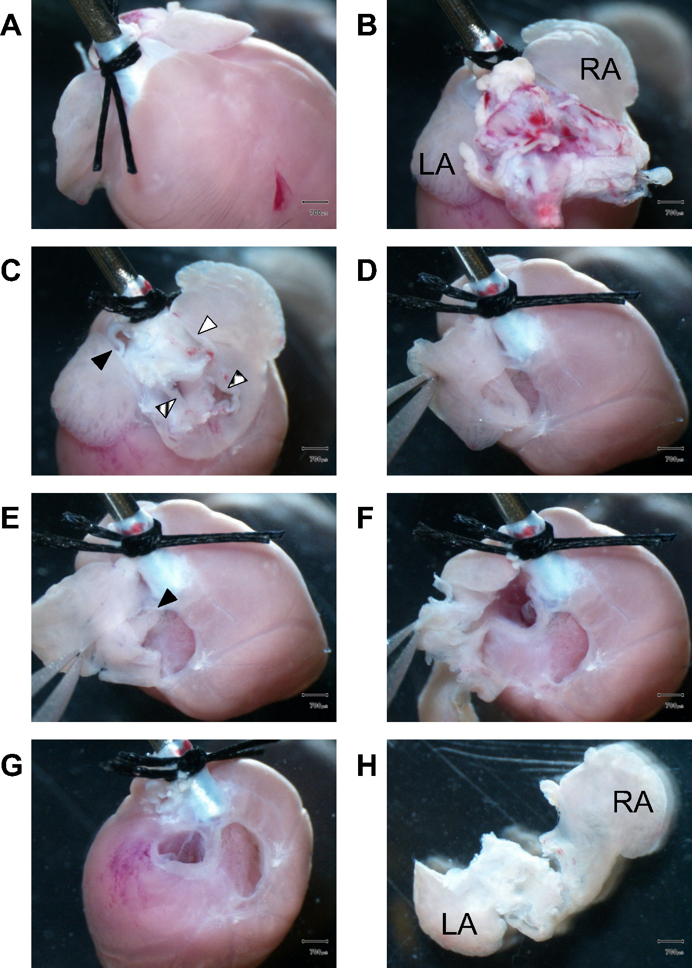
Figure 1.Dissection of atrial tissue. (A) Facing the anterior portion of the heart, two surgical sutures fix the proximal aorta to the stump end of a 21 G steel cannula. (B) View towards the heart basis shows remaining lung tissue obstructing the atrial chamber view during dissection. LA, left atrium; RA, right atrium. (C) Remaining lungtissue and great vessels were removed to access the atrial chambers. Filled black triangle, pulmonary artery; striated triangle, pulmonary veins; filled white triangle, upper vena cava; boxed triangle, lower vena cava. (D) First, the right atrial wall is dissected while the forceps hold the atrial appendage. (E) View into the right atrial chamber cavity. The black triangle marks the intact interatrial septum. (F) The dissection is continued to enter the left atrial chamber cavity. (G) Following complete dissection of the left and right atria, the atrioventricular valves become visible. The fibrous valve apparatus is dissected and discarded to subsequently harvest only ventricular muscle tissue. (H) Posterior view of the isolated left and right atria. LA, left atrium; RA, right atrium.Scale bars: 700 µm.

To determine the quality of cell isolations, Figure 2 provides typical cell examples during assessment of the yield and viability of typical rod or brick shaped striated intact myocytes, both for AMs and VMs. Little damaged, visually inconspicuous as well as severely damaged cells with abnormal excessively curved morphologies, or abnormal spherical shaped cells, can be readily identified including trypan blue exclusion as described in section 1.11. While intact myocytes remain bright and homogenously striated when exposed to extracellular trypan blue, damaged cells typically show multiple membrane blebs and/or quickly accumulate trypan blue intracellularly indicating membrane damage. However, trypan blue by itself can harm cells through unnecessarily long incubation and immediate cell quality assessment is therefore mandatory. Examples of more obvious forms of cell damage like myofilament contracture or gross surface damage compromising cell integrity are shown in Figures 4Cand4D. Please click here to view a larger version of this figure.

Figure 2.Trypan blue exclusion cell staining. Isolated (A)AM and (B)VM cells are mixed in suspension with trypan blue and visualized by an inverted light microscope shown at 40Xmagnification. Note thatabnormal spherical cells in (A)and (B)taking up trypan blue, which indicatesmembrane leakage and structural damage. In contrast, the centralAM and VM cells with intact membranes exclude trypan blue as shown. Furthermore, note that intact AM and VM cells show sarcomere striations throughout their cell volume, nomembrane blebs, and sharp edges at the both lateral sides and both intercalated discs. Scale bars: 20 µm.

Following successful isolation, cell yields of VMs from 5 x 10⁵ to 10⁶ can be expected from a single mouse heart digestion. The yield of AMs is significantly lower in the order of 3 x 10³to 3 x 10⁴ rod-shaped, trypan blue excluding cells. In contrast to VM, AM isolations occasionally fail even in experienced hands. Step 1.11 summarizes procedures how to estimate the yield of isolated healthy cells in suspension. Additionally, determine the average cell dimensions through step 1.13 as shown in Figure 3 for individual AM or VM cell isolates or to compare AM versus VM cell populations side-by-side (as needed). Please click here to view a larger version of this figure.

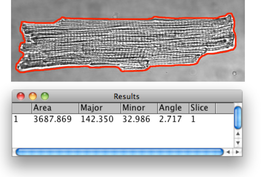
Figure 3.Bright field morphometric analysis of cardiac myocytes. The VM contour was detected by the image analysis tools described under step 1.13. Use the polygon selection tool to visually mark and define the cell extracellular border defined by the outer surface membrane for analysis. Ad the selected region of interest (ROI) to the ROI manager followed by 1D distance measurements. For comparative studies of AM vs. VM dimensions, it is useful to document the cell length, width, and area, and to calculate the length:width ratio.

To fluorescently stain TATS membranes either in AM or VM cells, the integral membrane dye di-8-ANEPPS is used as described in section 2 followed by confocal microscopy, which resulted in the representative images of TATS networks shown in Figures 4A and 4B. In addition, Figure 4A shows the corresponding transmitted light image of an intact AM side-by-side with the confocal TATS image (for image acquisition see section 3). As described by step 1.12, the morphological and surface membrane integrity of living myocytes is judged through the transmitted light images. The magnified region of the di-8-ANEPPS signal highlights the underlying morphology of the TATS network in AMs, characterized by abundant axial (longitudinal) membrane tubules. In contrast, the TATS morphology of healthy VMs as shown in Figure 4B is characterized by approximately similar numbers of axial and transverse components. In contrast, Figures 4C and 4D show examples of damaged cardiac myocytes that should be excluded from further analysis. In particular, the AM cell in Figure 4C is contracted as evidenced by an abnormally short sarcomere length of 1.2 µm and an irregular, distorted TATS network whereas the VM cell in Figure 4D exhibits multiple membrane blebs (some highlighted by red triangles) indicating membrane disruptions, which may occur at the outer surface membrane but also at the TATS membranes. Please click here to view a larger version of this figure.

Figure 4.Live membrane staining of intact atrial and ventricular myocytes. Corresponding transmitted light and confocal images of living di-8-ANEPPS stained intact (A)AM and (B)VM cells. In contrast, a partially contracted and potentially damaged AM with a sarcomere length of 1.2 µm is shown in (C). Contracted myocytes typically show abnormally shortened and distorted TATS structures, therefore excluded from further analysis. Another important indicator for cell membrane defects are membrane blebs (red triangles) as shown in a VM in (D). Membrane blebs represent damaged surface membrane structures and cells with blebs should be excluded from further TATS analysis. Furthermore, the VM shows gross damage apparently missing an entire part of its lower left portion (marked by asterisk). In summary, by comparing transmitted light and confocal images, cells morphology and surface intactness is documented and combined with fluorescent signal information. ‘N’ marks nuclei omitted from the analysis of the TATS membrane stain. Yellow bars indicate magnified ROIs from the same confocal image presented above. Scale bars: 10 µm. Please click here to view a larger version of this figure.

Confocal images of TATS membranes with a sufficient signal-to-noise ratio as shown in Figures 4A and 4B are accepted for further quantitative analysis. The TATS membrane analysis is based on skeletonized data derived from the fluorescent rectilinear signal components. Figure 5 shows the workflow diagram of the individual image processing steps which are described in detail by steps 4.3 to 4.5. These steps produce skeletonized images representing rectilinear TATS membrane networks as shown for each isolated VM (Figure 5A) and AM cells (Figure 5B).

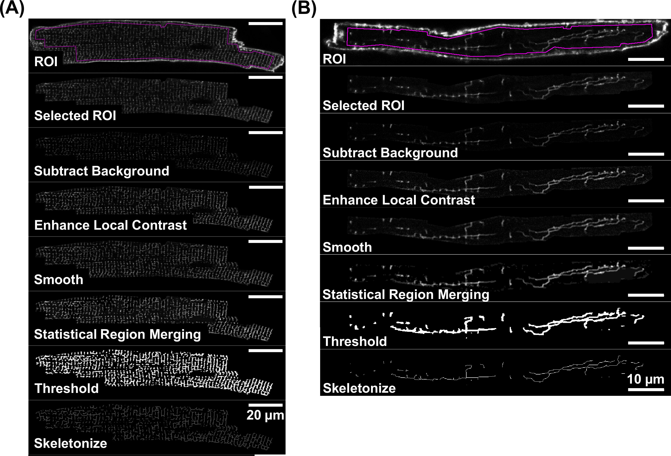
Figure 5.Workflow for skeletonization of fluorescent TATS images. Image processing steps which lead to a skeletonized image of the TATS network are represented by individual step-by-step image examples both for a di-8-ANEPPS stained VM (A)and AM (B). For individual image processing step, please refer to section 4. Note differences in scale bars: 20µm (A) and 10µm (B). Please click here to view a larger version of this figure.

A critical step during image processing, determine the appropriate threshold for data binarization as described in section 4.5.6. The resulting binary image should include only true membrane signals from the TATS network but not false structures derived by erroneous thresholding from the background signal noise. Yet, it is important that the threshold is low enough to detect all true TATS structures such that true TATS components are not erroneously lost during image analysis. Figure 6 illustrates the process how to select the threshold during data binarization. While a threshold of 40 as shown in Figures 6B and 6C seems appropriate to detect all true TATS structures individually, choosing a higher threshold e.g., of 60 as shown in Figure 6A does not detect fainter axial membrane structures (ATs) as indicated by yellow triangles. In contrast, choosing a lower threshold e.g., of 20 as shown in Figure 6D leads to erroneous detection of background noise as false-positive TATS structures as indicated by yellow triangles.

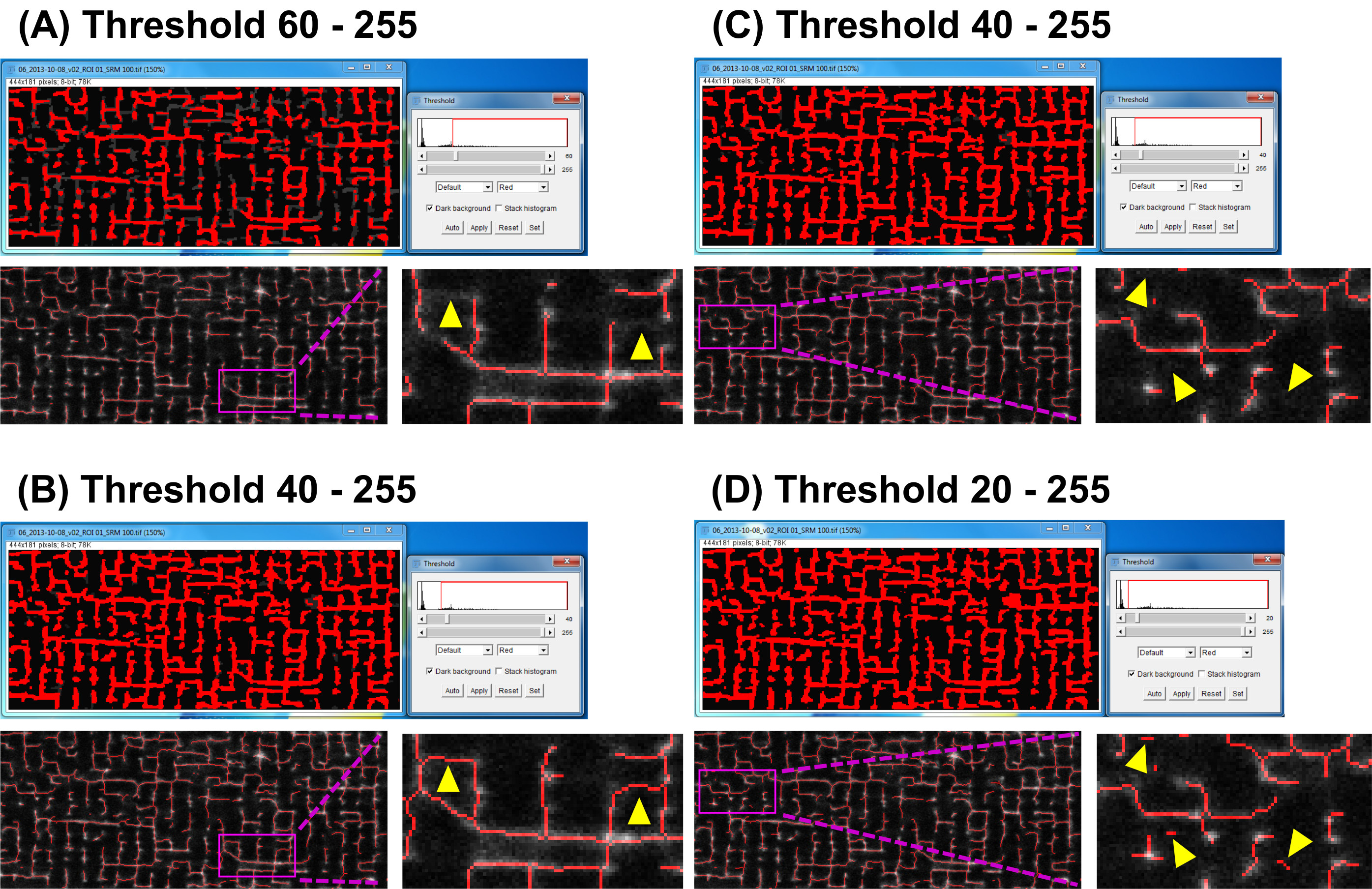
Figure 6.How to determine the signal threshold during skeletonizing of TATS image data. The examples show TATS skeletons each generated for different thresholds during data binarization (described in step 4.5). Upper images: show the threshold adjustments using Fiji. Lower images: overlay of skeletonized images with the corresponding input fluorescence image and magnified regions as indicated. A high threshold e.g., 60 applied in (A)is apparently not appropriate to detect all true TATS structures as indicated by yellow triangles in the magnified section. A threshold of 40 applied in (B)and (C)detects all TATS structures and correctly does not detect background noise, whereas a low threshold e.g., 20 in (D)erroneously identifies background noise as TATS structures and thereby produces false-positive signals of non-existing membrane structures. False-positive signals are indicated by yellow triangles in the magnified inset. Please click here to view a larger version of this figure.

The “Analyze Skeleton (2D/3D)” plugin supports the detailed analysis of skeletonized TATS structures. Once executed, the plugin produces a data table with the following skeleton parameters: #branches, #junctions, #end-point voxels, average branch length, #triple points, #quadruple points, and maximum branch length. For a detailed description of all possible output parameters please refer tohttp://fiji.sc/wiki/index.php/AnalyzeSkeleton and related articles^29-31. A typical data table output is shown in Figure 7A.

The parameters can be further used to derive the total skeleton length per area or the number of junctions per area. Exemplary calculation of the number of branches multiplied by the average branch length gives the total length of the continuous skeleton in 2D:

Total skeleton length per ROI:

∑ (#branches x average branch length)= 5155 px = 515.5 µm

The total length of the skeleton can be normalized to the image area. For the example shown in Figure 7 the normalized skeleton length of 0.64µm/µm² and the sum of all junctions are calculated as shown below:

Normalized skeleton length:

515.5 µm / 803.6 µm²= 0.64 µm/µm²

Normalized number of junctions:

155 junctions / 803.6 µm²= 0.19 junctions/µm²

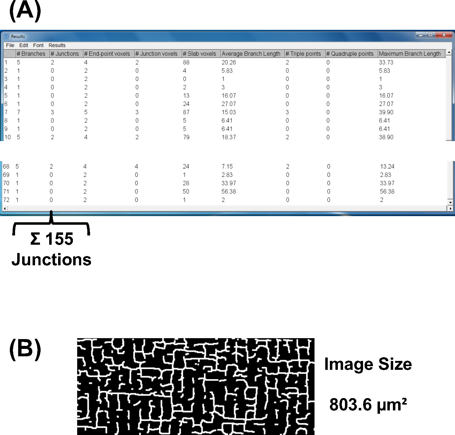
Figure 7.Automated data output from skeletonized images. (A) A typical data spreadsheet generated by the 'Analyze Skeleton (2D/3D)' plugin from the skeletonized image shown in (B). For a detailed description of possible output parameters please refer to http://fiji.sc/wiki/index.php/AnalyzeSkeleton. Please click here to view a larger version of this figure.

The image processing steps described under 4.5 and illustrated in Figure 5 can be automated using a Fiji macro provided as Supplementary Code File. The commands define repeats of image processing through reiterative steps. The macro can be applied to complete stacks of input images produced through steps 4.3 and 4.4. The macro can be advantageous for the analysis of complete dataset groups, for instance by preparing individual input image stacks for each independent treatment group for automated analysis using the macro commands.

The outlined software strategy further enables the TATS network orientation analysis for all components. For this, use the “Directionality” plugin (http://fiji.sc/Directionality)^29,31 which produces histogram data showing the orientation distribution of all TATS component orientations. If the x-axis of the input image corresponds to the main axis of a given AM or VM cell, the axial (longitudinal) TATS components will be represented by the 0° bin, whereas the transversal components will be represented by the 90° bin. Figure 8 shows exemplary directionality histograms from skeletonized TATS images for a VM (8A) versus an AM (8B) cell. While the directionality histogram of a typical VM shows a double peak distribution at 0° and 90°, the AM histogram shows a single dominant peak at 0°. These examples are in agreement with earlier observations that individual TATS components of VMs are nearly equally distributed between T-tubules and A-tubules, whereas the TATS components in AMs may be predominantly composed of A-tubules.

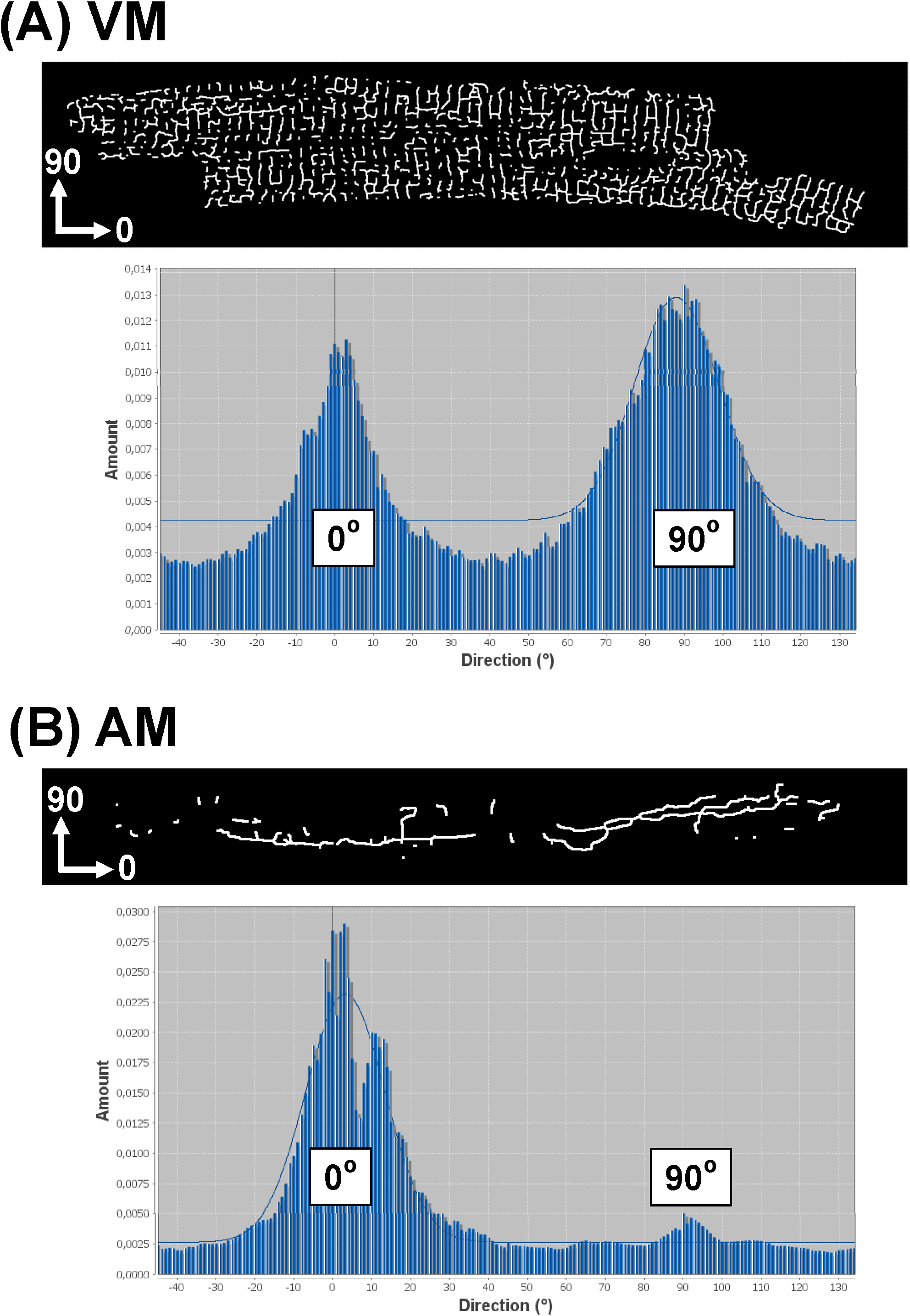
Figure 8.Representative directionality histogram from TATS networks of individual cells. Directionality histograms were generated from skeletonized images of individual VM (A)versus AM (B)TATS networks. Given that the x-axis of the analyzed image corresponds to the main (longitudinal) axis of the myocyte as shown, A-tubule components are represented by the 0° bin, whereas T-tubule components are represented by the 90° bin. Gauss fits only to the major histogram peakasshown as background graph. Please click here to view a larger version of this figure.

Perfusion buffer	mM
NaCl	120.4
KCl	14.7
KH2PO4	0.6
Na2HPO4	0.6
MgSO4	1.2
HEPES	10
NaHCO3	4.6
Taurine	30
2,3-Butanedione-monoxime	10
Glucose	5.5
pH 7.4
Digestion buffer	mM (if not specified)
NaCl	120.4
KCl	14.7
KH2PO4	0.6
Na2HPO4	0.6
MgSO4	1.2
HEPES	10
NaHCO3	4.6
Taurine	30
2,3-Butanedione-monoxime	10
Glucose	5.5
Collagenase type II	600 U/ml
pH 7.4
Stop buffer	mM (if not specified)
NaCl	120.4
KCl	14.7
KH2PO4	0.6
Na2HPO4	0.6
MgSO4	1.2
HEPES	10
NaHCO3	4.6
Taurine	30
2,3-Butanedione-monoxime	10
Glucose	5.5
CaCl2	0.0125
bovine calf serum	10%
pH 7.4

Table 1.Buffer solutions. The content of three different physiological buffer solutions for cell isolation and imaging are summarized.

Discussion

Although cardiac myocytes have been isolated and studied for decades³², a recent review concluded that consistent high-quality myocyte cell isolations remain challenging²⁷. This reflects relatively complex protocols for isolation of primary cardiac myocytes vis-à-vis a lack of common standard approaches, shared metadata, and transparent cell quality documentation. Cell isolation protocols are usually customized by individual groups, produce variable outcomes of cell isolates, depend on individual model settings (e.g., species, age, coexisting heart conditions), and are usually adjusted for particular experimental conditions. Within the context of the quantitative TATS membrane studies and protocols presented here, an essential level of quality assessment and documentation concerns the confocal or superresolution microscopy of individual cell membrane structures prone to metabolic and isolation protocol dependent changes, both in AM or VM. Importantly, even if high yields of cell isolates suggest healthy intact myocytes, investigators need to document and critically judge each individual cell carefully against morphological criteria of surface and TATS membrane integrity versus non-specific damage due to isolation procedures versus specific changes due to different types of interventions as compared to control conditions. An important variable during cardiac cell isolation is the specific activity of a given collagenase lot. To select a new lot of collagenase, the enzymatic activity of several collagenase samples should be tested against each other by evaluating cardiac myocyte yield and quality, and according to manufacturer instructions. Ideally, a new lot of collagenase is identified with collagenase activity similar to previous successfully used lots (for extended evaluation of possible enzyme activities refer to the “collagenase lot selection tool” in the materials and methods table). Taken together, quantitative approaches of TATS membrane visualization depend critically on cell isolation quality and, vice versa, cardiac cell isolations leading to unspecific membrane damage as documented by TATS microscopy should trigger critical review and correction of the isolation procedures. Since cell isolation quality and TATS membrane visualization and quantification are intrinsically linked, the protocols discussed in this article cover all major aspects as a continuous strategy.

An additional challenge and common issue of cardiac studies, cell damage and/or cell loss occur due to metabolically compromising interventions e.g., following myocardial infarction⁹, yet need to be judged against potential inadvertent damage e.g., following unnoticed air embolism during cell isolation. Isolation of cardiac myocytes from diseased hearts may lead to additional, significant cell loss and decreased cell yields. Therefore, comparison of the total number of isolated intact cells between control and diseased hearts can be meaningful if cell isolation and counting are consistently applied through standardized protocols. Consequently, it is critical to judge cell integrity through an appropriate control group, which reflects the best possible myocyte cell isolation quality. Importantly, individual cell quality and live cell microscopy of healthy versus diseased versus myocytes inadvertently damaged by the isolation procedure may significantly influence the analysis of TATS membrane networks. The protocols presented here therefore emphasize the integrity and stability of physiological membrane components during cell isolation and live cell microscopy of intact membranes. The entire workflow is designed as a continuous strategy to achieve and preserve intact TATS membrane components while excluding damaged cells, since these will exhibit isolation dependent membrane artifacts like disrupted membrane tubules, membrane blebs, and altered TATS networks erroneously under control conditions and compromise further quantitative analysis. Vice versa, the same strategies are crucial for intervention studies with the potential to disrupt TATS membranes, which depend critically on meaningful comparison controls between true healthy versus true diseased cell with TATS membrane changes.

In addition, we address procedures to achieve the technically much more challenging isolation of AM cells. Despite progress and improved protocols, it is important to emphasize that it is not trivial to reproduce high quality cell isolations of VMs and even less reliable for AMs. This is due to the overall lower yield of AM cells where even small errors or variations during cell isolation may lead to complete failure of AM cell isolation, whereas a mild degree of VM cell damage might be less apparent in cell suspension due to relatively high cell numbers compared to AM. Since AM cells might become curved after isolation, analysis through several ROIs can be advantageous as outlined under step 4.3. Following a detailed procedure of cell isolation steps, we provide a protocol for direct integral membrane staining and confocal or STED superresolution imaging of TATS networks both for VMs and AMs. These protocols enable both quantitative analysis and differentiation of select components of TATS membranes through previously established parameters. As compared to VMs, the 3D organization and functional behaviors of the atrial TATS network in AMs are currently less understood.

The procedures to image TATS membranes in living cells (steps 3.1 to 3.7) were developed with commercial confocal (Table of Materials/Equipment) and custom-made STED fluorescence microscopes⁹. To optimize the microscope settings for fluorescent image generation and quantitative TATS analysis, the following points are of general importance:

• Objective
  In order to resolve small details of TATS membrane structures, empirically test which objective provides the highest image quality while focusing several micrometer deep in the cell. Certain confocal microscopes may perform better with water or glycerol objectives, in contrast to the 63X 1.4 NA oil objective used here. Objectives with 100X magnification are used for superresolution STED microscopy, trading off a smaller field of view for nanometric resolution³⁴.
• Excitation and Gain
  The optimal settings of the excitation power and detector gain depend on the microscope light path, laser performance, and sample properties. Ideally, laser power and gain are adjusted to exploit the full range of the detector, yet avoid image saturation. Commercial microscopy software packages usually provide lookup tables that visualize the lower and upper limit of the dynamic range. Furthermore, to minimize dye bleaching employ the lowest possible laser power that still provides sufficient structural TATS membrane details. Also, excitation power should be low enough to avoid cumulative photo damage leading to myocyte contractures and death.
• Pixel Size
  Use a pixel size compatible with Nyquist sampling, approximately half the resolution achieved with the given settings. For confocal imaging a pixel size of 100 nm x 100 nm is compatible, which will also limit bleaching. For superresolution microscopy significantly smaller pixel sizes are used e.g., 20 nm x 20 nm for STED microscopy⁹.
• Dwell Time
  Confocal microscopes provide an averaging function. In general, use the shortest possible pixel dwell time to avoid bleaching in combination with signal averaging e.g., line-averaging ≥ 8 to improve the signal-to-noise-ratio.
• Document the Applied Microscopy Settings Through Meta-data
  Once the settings how to image details of TATS membrane structures were optimized on a particular confocal microscope, safe and/or document the settings (protocol meta-data). Acquire all images within a (or between) group(s) of cells with the same objective, excitation power, gain, pixel size, pixel dwell time, and averaging function. Equal imaging conditions allow for direct comparison and quantitation within a (or between) group(s) of cells.
• For general guidance and further details about principles and applications of confocal microscopy refer to the Handbook of Biological Confocal Microscopy (Pawley J.B., 3^rd Edition, 2006, Springer Science+Business Media, LLC).

In contrast to the direct analysis strategies presented here, previous publications describing TATS membranes and disease related changes, have used regional aggregate readouts of T-tubule density as quantitative strategy^16,17, or indirect regional strategies based on Fourier transformation analysis of striated membrane signals in order to assess T-tubule component regularity⁷. In contrast, the quantitative approaches described here are directly related to individual TATS components and provide a number of additional parameters including membrane network properties and specific components like the percentage of A-tubules. Furthermore, the TATS network density can be quantified as the normalized length of the entire extracted skeleton per ROI area. The number of triple junctions of three individual, continuously connected tubule components can be used as a measure of the branching complexity of the TATS membrane network. We note that any analysis of smallest TATS components depends on the staining procedures. In our experience, 800 µl of a 50 µM di-8-ANEPPS solution are sufficient to stain complete TATS networks in a cell pellet containing 50,000 VM cells⁹. However, if the cell pellet contains a lower number of cardiac myocytes, if powerful fluorescence detectors are available, and if confocal imaging of the overall TATS network distribution rather than smallest membrane details and quantitative changes are of interest, lower dye concentrations may be used based on empirical testing. Finally, a software macro written for the described analysis can be used to automate the image processing steps to facilitate analysis of larger datasets, which is particularly useful for comparison between different treatment groups (e.g., drugs), cell types (e.g., AM versus VM), and pathophysiological interventions (e.g., sham versus myocardial infarction).

For image analysis of TATS networks, the following sequence of principle steps is applied: 1) rolling ball background–subtraction (4.5.1) to remove spatial variations in background intensity; 2) local contrast enhancement (4.5.2.); 3) image smoothing (4.5.3); 4) statistical region merging (4.5.4); 5) defining the threshold of image binarization (4.5.6); and 6) calculation of the skeleton data (4.5.8). A critical step during the skeletonization of fluorescent TATS images is the image binarization shown in Figure 6. The associated thresholding steps ultimately define which true membrane structures are detected to represent the underlying TATS components versus potentially false structures identified by error from background noise. Identification of the correct threshold for binary image analysis should correspond with the true TATS membrane structures, which depends on a sufficiently high signal-to-noise (SNR) ratio each for confocal and superresolution microscopy approaches. Therefore, a sufficient image quality should be established first and subsequently combined with critical judgment of individual cell quality including documentation by bright field images as outlined. Alternative options to adapt the image segmentation protocol for a given microscope data output and/or physiological questions include image deconvolution and other thresholding procedures like “Otsu” or “Iso-data” available as ImageJ plugins. Regardless of the final segmentation procedure, we consider the comparison between extracted and raw data by image overlay a mandatory quality control step. In summary, morphological and membrane integrity of individual isolated myocytes, sufficient staining of intracellular TATS membranes, parameter optimization for fluorescence imaging, and overlay control of extracted skeleton data will all contribute to the quality of fluorescent TATS images and quantitative results.

If larger species than mouse are used for cell isolation, the protocols can be readily adapted as appropriate. For the next larger species, rat hearts can be cannulated with a blunt 14 G cannula (outer diameter 2.1 mm) and perfused at 8 ml/min. Significantly older or diseased hearts may require even larger cannula sizes. In general, cardiac perfusion may be conducted either by constant pressure e.g., using a 1 m high water column between reservoir and aorta or by constant flow using a peristaltic pump. For cell isolation from small rodent hearts like mice and rats constant flow may be advantageous since collagenase digestion will eventually disrupt coronary resistance vessels leading to excessive perfusion rates from leaking vessel beds which will be controlled to some degree by constant flow protocols. In contrast, constant pressure perfusion is advantageous if monitoring of the flow rate and correct cannulation are a priority, which is advantageous for intervention models with altered blood vessel resistance behaviors as well as for training of the cell isolation procedures.

As outlined above, sufficient cell quality is very important for quantitative studies of endogenous membrane systems. However, during heart perfusion and collagenase digestion numerous factors can critically affect the quality of the cell isolation, which should never be underestimated during protocol optimization or trouble shooting²⁷. In particular, the activity of a given collagenase lot should be determined for the specific tissue of interest e.g., atria or ventricles prior to execution of the experimental bona fide studies to establish isolation conditions to be maintained throughout the remainder of the study. Furthermore, the water quality, pH, temperature, optimization and cleaning of the perfusion setup will minimize the risk of inadvertent damage from contaminants and emboli, and potentially additional factors have to be monitored to establish optimal homeostatic conditions during cell isolation. BDM (2,3-butanedione-monoxime) a reversible inhibitor of myosin ATPase cross-bridges is commonly used during tissue dissection and digestion to sustain cardiac muscle relaxation, which increases the yield of cell isolations. Nevertheless, investigators need to be aware that BDM may exert non-specific phosphatase activities leading to off-target effects e.g., inhibition of Na⁺/Ca²⁺ exchange currents under certain conditions³³. For some experiments it might be advantageous to replace BDM by blebbistatin as cardioplegic solution, an inhibitor with a high affinity for myosin at micromolar concentrations which is, however, toxic and relatively expensive and may have other off-target effects. Resting healthy cardiomyocytes should not show any contractions in the absence of electrical stimulation and such cells should be excluded from further analysis. On the other hand, cardiac myocyte contraction and relaxation in response to electrical stimulation at physiological extracellular Ca²⁺ concentrations can be used to establish normal contractile behavior as an additional measure to assess functional cell quality and/or abnormal behavior in heart disease versus healthy control cells.

In summary, the protocols for single cell isolation and quantitative image analysis described here have been successfully applied for confocal and superresolution microscopy of the TATS membrane network in VM⁹ and AM cells²¹ as well as for quantitative analysis of microtubule networks in fixed cardiac myocytes (data not shown). These and future applications of the protocols may open avenues for a variety of experimental questions such as the characterization of TATS membranes at different developmental stages or the analysis of membrane associated protein or organelle structures that contact the TATS network to exert highly localized, domain specific signaling functions in AM and VM cells.

Materials

List of materials used in this article

Name	Company	Catalog Number	Comments
Chemicals and Enzymes
2,3-Butanedione monoxime	Sigma-Aldrich, Munich, Germany	B0753
Bovine calf serum	Thermo Scientific, Schwerte, Germany	SH30073	Triple 0.1 µm sterile filtered.
CaCl2	Sigma-Aldrich, Munich, Germany	21115	Diluted 1:10 in MQ water to obtain 100 mM CaCl2 stock concentration.
Collagenase type II	Worthington via Cell Systems, Troisdorf, Germany	on request	Enzymatic activity depends on individual collagenase batches. Collagenase II and other enzyme activities (Caseinase, Clostripain, Tryptic) can be assessed in the "collagenase lot selection tool". Determine cell yield and quality individually for each new lot of collagenase.
Glucose	Carl Roth, Karlsruhe, Germany	HN06.1
Heparin	Rotexmedica, Trittau, Germany	PZN-03862340	Diluted in 0.9% NaCl and injected subcutaneuosly in abdominal skin.
HEPES	Carl Roth, Karlsruhe, Germany	9105.4
Forene 100% (V/V)	Abbott, Libertyville, IL, USA	B506	Active agent: isoflurane, 250 ml. Use approximately 2 Vol% in air/oxygen dispenser instrument.
KCl	Carl Roth, Karlsruhe, Germany	6781.3
KH2PO4	Carl Roth, Karlsruhe, Germany	3904.2
Laminin (2 mg/ml)	BD Biosciences, Heidelberg, Germany	354232	Lamination is described under step 2.1.
MgCl2·6H2O	Carl Roth, Karlsruhe, Germany	2189.2
MgSO4·7H2O	Carl Roth, Karlsruhe, Germany	8283.2
Na2HPO4·2H2O	Carl Roth, Karlsruhe, Germany	4984.2
NaHCO3	Carl Roth, Karlsruhe, Germany	HN01.1
Taurin	Carl Roth, Karlsruhe, Germany	4721.2
Dyes
Di-8-ANEPPS	Molecular Probes, Life Technologies, Darmstadt, Germany	D-3167	Stock solution 2 mM in DMSO
Trypan blue	Sigma-Aldrich, Munich, Germany	T8154	Trypan blue is gently mixed 1:1 via tip-cut 1 ml plastic pipette with cell suspension prior to cell counting in Neubauer cytometer.
Langendorff Perfusion Setup
Circulation thermostat	Lauda, Lauda-Königshofen, Germany		Please refer to Louch et al. (JMCC 2011). Heat up thermostat und buffers in perfusion tubing to 37 °C 15 min prior to use.
Flexible silicone tubing Tygon for peristaltic pump	VWR, Darmstadt, Germany	224-2252	Tubing needs to be changed regularly.
Flexible silicone tubing Tygon for thermostat	VWR, Darmstadt, Germany	228-4340
Heating coil surroundung perfusion tubing	Rettberg, Göttingen, Germany	custom-made	Heating coil and tubing needs to be cleaned thoroughly via MQ water after using. Do not use detergents. Glass components should be bathed regularly  in 10 mM NaOH overnight.
Peristaltic pump	Ismatec, Wertheim, Germany	ISM830
Three way stop cock Discofix C Luer Lock 10 cm	Braun, Melsungen, Switzerland	16500C
Three way stop cock Discofix 3SC	Braun, Melsungen, Switzerland	4095146
Instruments
42 mm glass coverslips	Menzel Gläser via Thermo Scientific, Schwerte, Germany	on request	0.13-0.16 mm thickness
Cannula 21 G	Becton, Dickinson and Company, Franklin Lake, NY, USA	304432	Cut to a length of ~5 mm, roughened with sandpaper.
Coverslips for Neubauer cytometer 24 x 24 mm	Menzel Gläser via Thermo Scientific, Schwerte, Germany	on request	0.38-0.42 mm thickness
Graefe forceps, 0.5 mm tips, slight curve	Fine Science Tools, Heidelberg, Germany	11151-10
LSM 710 NLO	Carl Zeiss, Jena, Germany		63X 1.4 NA oil objective
Neubauer improved cytometer	Labor Optik, Friedrichsdorf, Germany	1100000	Counting procedure: Wipe cytometer and coverslip provided with the counting chamber with 70 % ethanol. Press coverslip gently on the counting chamber so that the two glass surfaces are in contact and Newton's rings can be observed. Subsequently, 10-20 µl cell suspension can be applied to the edge of the coverslip to be sucked into the void by capillary action. Count the intact vs. defect myocytes using the squares of the cytometer grid which reflects 100 nl. Repeat counting procedure on the second grid provided on the cytometer. Calculate the density of cells in your original cell suspension by taking account of any dilutions and counting shortcuts.
POC-R2 Imaging Chamber	Pecon, Erbach, Germany		Cell suspension volume: 800 µl; desired plating density: ~1,000 AM and ~10,000 VM
Spring scissors, 8 mm blades straight, blunt	Fine Science Tools, Heidelberg, Germany	15025-10
Student dumont #7 forceps, inox	Fine Science Tools, Heidelberg, Germany	91197-00
Student iris scissors, curved, 11.5 cm	Fine Science Tools, Heidelberg, Germany	91461-11
Student iris scissors, straight, 11.5 cm	Fine Science Tools, Heidelberg, Germany	91460-11
Student surcigal scissors, straight, sharp, 12 cm	Fine Science Tools, Heidelberg, Germany	91402-12
Tissue forceps, 1 x 2 teeth, slim, 10 cm	Fine Science Tools, Heidelberg, Germany	11023-10

References

- Prosser, B. L., Ward, C. W., Lederer, W. J. Subcellular Ca2+ signaling in the heart the role of ryanodine receptor sensitivity. J Gen Physiol. 136 (2), 135-142 (2010).
- Wehrens, X. H., Lehnart, S. E., Marks, A. R. Intracellular calcium release and cardiac disease. Annu Rev Physiol. 67, 69-98 (2005).
- Cheng, H., Cannell, M. B., Lederer, W. J. Propagation of excitation-contraction coupling into ventricular myocytes. Pflugers Arch. 428 (3-4), 415-417 (1994).
- Williams, G. S., Chikando, A. C., Tuan, H. T., Sobie, E. A., Lederer, W. J., Jafri, M. S. Dynamics of calcium sparks and calcium leak in the heart. Biophys J. 101 (6), 1287-1296 (2011).
- Sperelakis, N., Rubio, R. orderly lattice of axial tubules which interconnect adjacent transverse tubules in guinea-pig ventricular myocardium. J Mol Cell Cardiol. 2 (3), 211-220 (1971).
- Soeller, C., Cannell, M. B. of the transverse tubular system in living cardiac rat myocytes by 2-photon microscopy and digital image-processing techniques. Circ Res. 84 (3), 266-275 (1999).
- Song, L. S., et al. et al. ryanodine receptors in the failing heart. Proc Natl Acad Sci USA. 103 (11), 4305-4310 (2006).
- Oort, R. J., et al. Disrupted junctional membrane complexes and hyperactive ryanodine receptors after acute junctophilin knockdown in mice. Circulation. 123 (9), 979-988 (2011).
- Wagner, E., et al. Stimulated emission depletion live-cell super-resolution imaging shows proliferative remodeling of T-tubule membrane structures after myocardial infarction. Circ Res. 111 (4), 402-414 (2012).
- Asghari, P., Schulson, M., Scriven, D. R., Martens, G., Moore, E. D. Axial tubules of rat ventricular myocytes form multiple junctions with the sarcoplasmic reticulum. Biophys J. 96 (11), 4651-4660 (2009).
- Lukyanenko, V., Ziman, A., Lukyanenko, A., Salnikov, V., Lederer, W. J. Functional groups of ryanodine receptors in rat ventricular cells. J Physiol. 583 (Pt 1), 251-269 (2007).
- Shacklock, P. S., Wier, W. G., Balke, C. W. Local Ca2+ transients (Ca2+ sparks) originate at transverse tubules in rat heart cells. J Physiol. 487 (Pt 3), 601-608 (1995).
- Reynolds, J. O., et al. Junctophilin-2 is necessary for T-tubule maturation during mouse heart development. Cardiovasc Res. 100 (1), 44-53 (2013).
- Di Maio, A., Karko, K., Snopko, R. M., Mejia-Alvarez, R., Franzini-Armstrong, C. T-tubule formation in cardiac myocytes two possible mechanisms. J Muscle Res Cell Motil. 28 (4-5), 231-241 (2007).
- He, J., et al. Reduction in density of transverse tubules and L-type Ca(2+) channels in canine tachycardia-induced heart failure. Cardiovasc Res. 49 (2), 298-307 (2001).
- Heinzel, F. R., et al. Remodeling of T-tubules and reduced synchrony of Ca2+ release in myocytes from chronically ischemic myocardium. Circ Res. 102 (3), 338-346 (2008).
- Lyon, A. R., et al. Loss of T-tubules and other changes to surface topography in ventricular myocytes from failing human and rat heart. Proc Natl Acad Sci USA. 106 (16), 6854-6859 (2009).
- Crossman, D. J., Ruygrok, P. N., Soeller, C., Cannell, M. B. Changes in the organization of excitation-contraction coupling structures in failing human heart. PLoS One. 6 (3), e17901(2011).
- Kemi, O. J., et al. The effect of exercise training on transverse tubules in normal, remodeled, and reverse remodeled hearts. J Cell Physiol. 226 (9), 2235-2243 (2011).
- Sachse, F. B., et al. Subcellular structures and function of myocytes impaired during heart failure are restored by cardiac resynchronization therapy. Circ Res. 110 (4), 588-597 (2012).
- Arakel, E. C., et al. Tuning the electrical properties of the heart by differential trafficking of KATP ion channel complexes. J Cell Sciences. 127 (Pt 9), 2106-2119 (2014).
- Richards, M. A., et al. Transverse tubules are a common feature in large mammalian atrial myocytes including human. Am J Physiol Heart Circ Physiol. 301 (5), H1996-H2005 (2011).
- Trafford, A. W., Clarke, J. D., Richards, M. A., Eisner, D. A., Dibb, K. M. Calcium signalling microdomains and the t-tubular system in atrial mycoytes potential roles in cardiac disease and arrhythmias. Cardiovasc Res. 98 (2), 192-203 (2013).
- Greiser, M., Schotten, U. Dynamic remodeling of intracellular Ca2+ signaling during atrial fibrillation. J Mol Cell Cardiol. 58, 134-142 (2013).
- Voigt, N., Zhou, X. B., Dobrev, D. Isolation of human atrial myocytes for simultaneous measurements of Ca2+ transients and membrane currents. J Vis Exp. (77), 10-3791 (2013).
- Kaestner, L., et al. Isolation and genetic manipulation of adult cardiac myocytes for confocal imaging. J Vis Exp. (31), (2009).
- Louch, W. E., Sheehan, K. A., Wolska, B. M. Methods in cardiomyocyte isolation, culture, and gene transfer. J Mol Cell Cardiol. 51 (3), 288-298 (2011).
- King, N. M., et al. Mouse intact cardiac myocyte mechanics cross-bridge and titin-based stress in unactivated cells. J Gen Physiol. 137 (1), 81-91 (2011).
- Schindelin, J., et al. Fiji, an open-source platform for biological-image analysis. Nat Methods. 9 (7), 676-682 (2012).
- Arganda-Carreras, I., Fernandez-Gonzalez, R., Munoz-Barrutia, A., Ortiz-De-Solorzano, C. 3D reconstruction of histological sections Application to mammary gland tissue. Microsc Res Tech. 73 (11), 1019-1029 (2010).
- Liu, Z. Q. Scale space approach to directional analysis of images. Appl Opt. 30 (11), 1369-1373 (1991).
- Powell, T., Twist, V. W. A rapid technique for the isolation and purification of adult cardiac muscle cells having respiratory control and a tolerance to calcium. Biochem Biophys Res Commun. 72 (1), 327-333 (1976).
- Watanabe, Y., et al. Inhibitory effect of 2,3-butanedione monoxime (BDM) on Na(+)/Ca(2+) exchange current in guinea-pig cardiac ventricular myocytes. Br J Pharmacol. 132 (6), 1317-1325 (2001).
- Kohl, T., Westphal, V., Hell, S. W., Lehnart, S. E. Superresolution microscopy in heart - cardiac nanoscopy. J Mol Cell Cardiol. 58, 13-21 (2013).
Reprints and Permissions