Hybrid µCT-FMT imaging and image analysis

Summary

We describe a protocol for hybrid imaging, combining fluorescence-mediated tomography (FMT) with micro computed tomography (µCT). After fusion and reconstruction, we perform interactive organ segmentation to extract quantitative measurements of the fluorescence distribution.

Abstract

Fluorescence-mediated tomography (FMT) enables longitudinal and quantitative determination of the fluorescence distribution in vivo and can be used to assess the biodistribution of novel probes and to assess disease progression using established molecular probes or reporter genes. The combination with an anatomical modality, e.g., micro computed tomography (µCT), is beneficial for image analysis and for fluorescence reconstruction. We describe a protocol for multimodal µCT-FMT imaging including the image processing steps necessary to extract quantitative measurements. After preparing the mice and performing the imaging, the multimodal data sets are registered. Subsequently, an improved fluorescence reconstruction is performed, which takes into account the shape of the mouse. For quantitative analysis, organ segmentations are generated based on the anatomical data using our interactive segmentation tool. Finally, the biodistribution curves are generated using a batch-processing feature. We show the applicability of the method by assessing the biodistribution of a well-known probe that binds to bones and joints.

Introduction

Fluorescence-mediated tomography, also called fluorescence molecular tomography (FMT), is a promising technique to quantitatively assess the fluorescence distribution in diffuse tissues, such as anesthetized mice or even human body tissues, e.g., breasts or finger joints. In contrast to non-invasive microscopy techniques, which allow imaging of superficial targets at subcellular resolution¹, FMT allows three-dimensional reconstruction of fluorescent sources in depths of several centimeters, albeit at lower resolution². Many targeted fluorescent probes are available to image angiogenesis, apoptosis, inflammation, and others^2–5. Some probes are activatable, e.g., by specific enzyme cleavage leading to unquenching of fluorochromes. Moreover, reporter genes expressing fluorescent proteins can be imaged, e.g., to track tumor cell migration⁶.

FMT strongly benefits from the combination with an anatomical modality, e.g., µCT^2,7 or MRI⁸. While stand-alone FMT devices are commercially available⁹, the fluorescence images are difficult to interpret without anatomical reference information. Recently we were able to show, that the fused anatomical image data enables a more robust analysis¹⁰. The anatomical data can also be used to provide prior knowledge, such as the outer shape of the mouse, which is important for accurate optical modeling and fluorescence reconstruction¹¹. Furthermore, optical scattering and absorption maps can be estimated using segmentation of tissue types and by assigning class specific coefficients^12,13. For near-infrared light, hemoglobin is the main absorber in mice, besides melanin and fur¹⁴. Since the relative blood volume varies regionally by orders of magnitude, an absorption map is particularly important for quantitative fluorescence reconstruction¹³.

One advantage of using non-invasive imaging devices is that the mice can be imaged longitudinally, i.e., at multiple time points. This is important to assess the dynamic behavior of probes, i.e., their target accumulation, biodistribution and excretion^10,15, or to assess the disease progression¹⁶. When imaging several mice at multiple time points, a large amount of image data sets arises. To enable comparability, these should be acquired in a systematic way, i.e., with a well-defined and documented protocol. The large number of scans poses a challenge for image analysis, which is required to extract quantitative measurements from the image data.

The purpose of our study is to provide a detailed description of a µCT-FMT imaging protocol which we used and optimized throughout several studies^{10,13,15,17,18}. We describe how the data sets are generated, processed, visualized, and analyzed. This is demonstrated using an established molecular probe, OsteoSense, that binds to hydroxyapatite¹⁹, and can be used to image bone diseases and remodeling². All procedures involving animals were approved by the governmental review committee on animal care.

Protocol

The protocol contains a detailed description of the following steps: At first, phantoms or mice and the multimodal mouse bed are prepared for imaging. Then a whole-body scan is acquired in the µCT. Subsequently the mouse bed is transferred to the FMT where two scans are acquired (up and upside down). This can be repeated for multiple mice at multiple time points. After completion of the data acquisition, the data needs to be exported and sorted to enable automated segmentation (requiring a Definiens software license), as well as image fusion and fluorescence reconstruction (requiring an Imalytics Preclinical software license). Finally it is shown how the multimodal data sets are visualized and how organs are interactively segmented to quantify the biodistribution of fluorescent probes.

1. Phantom Preparation

NOTE: Phantoms are useful to test the imaging system, but also to determine the calibration factor for a new probe.

1. Prepare a solution of 200 ml water, 2 % agarose, 1.8 g TiO₂ powder, 50 µl trypan blue. After boiling, fill the solution into a rectangular form, approximately of 8 cm length, 3 cm width, and 1.5 cm height.
2. Prepare several fluorescent inclusions in the phantom using pipette tips, containing a mix of fluorescence and µCT contrast agent. To create the inclusions, cut the pipette tips and seal them with a lighter.
3. After the solution has solidified, insert the inclusions into the phantom. Cut away some parts of the phantom to achieve an irregular shape and to fit it to the multimodal mouse holder.
4. To determine the calibration factor for a new probe, some phantom scans are required. For this, the default FMT phantom is used in combination with known amounts of the probe. For an increased accuracy, add 4 % lipid emulsion to the solution to receive the same scattering coefficient inside the inclusion as in the rest of the phantom. Also add a small amount (2 %) of µCT contrast agent for easier image analysis.

2. Mouse Preparation

NOTE: µCT-FMT imaging requires special preparation including anesthetization and hair removal.

1. Place the mouse on chlorophyll-free food 7 days before imaging. This will reduce the background signal and is particularly important for FMT channels below 750 nm.
2. All animal experiments are performed under anesthesia. To initiate the anesthesia, place the mouse in a chamber filled with 2 % isoflurane in air (flow rate 5 L/min) until the mouse is falling asleep. Confirm proper anesthetization by gentle toe or skin pinching and by checking relaxation of muscle tonus (e.g., jaw muscle). To sustain the anesthesia, continue the isoflurane application using a tube that is placed on the nose of the mouse (2 % isoflurane in air, flow rate 1 L/min). In order to prevent eye dryness, use vet ointment on anesthetized mice.
3. To inject contrast agent, fix the anesthetized mouse on a heating pad using tape. Place a catheter (syringe needle attached to a tube) to the tail vein and inject the fluorescent contrast agent (e.g., 2 nmol, with maximal injection volume of 5 ml/kg body weight, i.e., 150 µl for a 30 g mouse).
4. For scanning a hairy mouse, the scanning area has to be depilated in advance. For this, use a shaver or hair removal cream. Some strains of mice can develop rashes from the hair removal cream. Therefore, monitor the mice for skin changes and contact veterinary staff for care if needed. Also test the tolerance on a small number of animals when using new mouse strains.
5. Keep the mouse anesthetized during µCT and FMT imaging (2 % isoflurane in air, flow rate 1 L/min).

3. Mouse Bed Preparation

NOTE: For µCT-FMT scanning, use a multimodal mouse bed, which fits both into the µCT and the FMT.

1. Before imaging, clean the mouse bed with wet tissues. Do not use ethanol because this may damage the acrylic glass. Make sure that the markers are free of water, because this may impair the automated marker detection.
2. Open the screws of the multimodal mouse bed and remove the upper part.
3. Attach the anesthetic gas tube on the mouse bed and fixate it with tape.
4. Place the anesthetized mouse into the mouse bed and put the nose into the gas tube. Make sure the head of the mouse is at the front indicator of the mouse bed (Figure 1).
5. Make sure that the mouse is in the middle of the mouse bed to optimally use the field of view of the FMT.
6. Close the mouse bed and tighten the screws until the mouse is tightly held. Make sure the mouse can breathe steadily by visual monitoring of thoracic breathing movements.

4. µCT Imaging

NOTE: A whole-body scan is performed using the µCT. The generated anatomical data is required for image fusion, for an improved fluorescence reconstruction and for image analysis.

1. Place the mouse bed with the mouse into the µCT. Make sure that the mouse is placed in a way that it goes “tail-first” into the µCT. This is important for the automated fusion.
2. In order to sustain anesthesia when the µCT-lid is closed, reconnect the tubes to channel the gas through the case of the µCT. First detach the long tube from the mouse bed and attach it to the connector at the outside of the µCT. Then attach the remaining free end to the connector inside the µCT.
3. Drive the mouse bed into the µCT. Make sure that the gas tube is not loose and cannot get caught by the rotating gantry. If necessary, fixate it with tape. Insert the tube into the cut-out of the holder of the mouse bed.
4. Close the µCT and acquire a topogram. Select at least two subscans to cover a substantial part of the mouse and the mouse bed, which is important for the fusion and reconstruction.
5. Select the µCT scan protocol named HQD-6565-360-90, which acquires 720 projections with 1032 x 1012 pixels during one full rotation requiring a scanning time of 90 s per subscan. Tubes are operated at voltage 65 kV and current 1.0 mA. Alternatively, to reduce the radiation dose and scanning duration, select the scanning protocol SQD-6565-360-29 which acquires 720 projections with 516 x 506 pixels with scanning time 29 s per subscan.
6. Start the µCT scan. The blue bar indicates the progress. The subscans will be acquired subsequently. Hypothermia and fluid loss are not a problem because of the short scanning duration of only a few minutes. Do not open the lid of the µCT during scanning because this will automatically interrupt the scanning to protect the user from radiation.
7. When the scanning is completed, open the lid, reconnect the anesthetic tube and detach the mouse bed from the holder to transport it to the FMT.

5. FMT Imaging

NOTE: Directly after µCT scanning, the mouse is scanned in the FMT in two configurations (up and upside down) which are used together for an improved fluorescence reconstruction.

1. Turn on the anesthetic gas supply (2 % isoflurane in air, flow rate 1 L/min) for the FMT before placing the mouse bed into the FMT. Using the FMT control software, create a study group with an appropriate number of subjects (i.e., mice). Select the probes that will be used for imaging (use OsteoSense for novel probes that are not listed).
2. Carry the multimodal mouse bed with the mouse to the FMT. The long flexible anesthetic gas tube maintains the gas flow. Before inserting the mouse bed into the FMT, carefully remove the tube since it is not needed inside the FMT. Avoid turning the screws of the mouse bed.
3. Place the mouse bed into the FMT with the red indicator first (“head-first”). This is important for the image fusion to be consistent with the µCT.
4. Close the FMT.
5. Select the correct study group and subject. Select the required channel of the FMT (for OsteoSense 750EX, use the 750 nm channel).
6. Add a description, e.g., “up” or “down” and acquire an overview scan by pressing “Capture”. This captures a reflectance image of the entire field of view. Make sure to not have “Reflectance Images Only” selected, because otherwise it is not possible to acquire 3D scans subsequently.
7. Adjust the imaging parameters for the 3D scan. Enlarge the field of view to include as much as possible of the mouse. Usually, the head and tail will not entirely fit into the field of view, however. Click “Advanced” and check the imaging settings. Set sampling density to 3 mm, sensitivity to normal and illumination min/max to 5000 and 50000, respectively.
8. Click “add to reconstruction queue” and then click “Scan” to start the FMT scan. This will take around 5 to 15 min, depending on the size and thickness of the mouse, because longer exposure times are required for thicker objects. The device contains a heated imaging chamber to avoid hypothermia.
9. After the scan, flip the mouse bed including the mouse upside down and acquire another scan. This provides additional data for the fluorescence reconstruction.
10. When the µCT and the FMT-scans are completed and the mouse wakes up from the anesthesia, do not leave it unattended until it has regained sufficient consciousness, e.g., to walk around or to maintain sternal recumbency.

6. Image Fusion and Reconstruction

NOTE: After completion of the µCT-FMT scanning, e.g., at the end of the study, the acquired data needs to be sorted to enable the automated image fusion and fluorescence reconstruction.

1. To sort the scans for further processing, create a folder for the study. For each µCT-FMT scan, create one subfolder whose name contains the mouse ID and the time point, e.g., M01_02h.
2. For each µCT-FMT scan, export the FMT scans (up and down) as .fmt files and save them into the subfolder using filenames ending with either “_up.fmt” or “_down.fmt”. Each .fmt file contains the acquired raw data, i.e., the excitation and emission images acquired by the camera, the metadata, such as the exposure times, and the fluorescence reconstruction generated by the FMT.
3. Using the µCT software, create a reconstruction with isotropic voxel size 35 µm. Select a smooth reconstruction kernel (T10). Adjust the field of view so that the entire mouse bed including the markers is covered. Select MIFX/RAW as output format and start the reconstruction. After the reconstruction is done, move the µCT reconstruction files into the subfolder of the µCT-FMT scan.
4. Export the µCT and FMT data for all scans. Make sure that each subfolder contains two .fmt files (up and down) and the µCT reconstruction in the MIFX/RAW format. To check for completeness select Menu->CT-FMT->Check Completeness using the Imalytics Preclinical software. A list of errors might appear, such as missing .fmt files or µCT reconstructions. Fix the errors and check for completeness until all errors are resolved.
5. Using Menu->CT-FMT->Settings, check the server name of the Definiens software and adjust if necessary. The default is http://localhost:8184, assuming that the Definiens software is installed on the same computer. The Definiens software is required in the next step to perform the automated segmentation of the mouse bed and markers.
6. Click Menu->CT-FMT->Fuse group in the Imalytics Preclinical software to perform automated µCT-FMT fusion for the entire study. This takes a few minutes per µCT-FMT scan and results in a folder with suffix “Package” parallel to the study folder. This contains a smaller subset of files (the µCT data and the fused vendor-provided FMT reconstruction) that are relevant for further analysis.
7. Click Menu->CT-FMT->Reconstruct group (FMT) in the Imalytics Preclinical software to perform the fluorescence reconstruction including the generation of absorption and scattering maps¹³. Even though the processing is GPU-accelerated²⁰, each reconstruction requires 1 to 4 hr depending on the size of the mouse. The results will be stored in the package folder. Note: To enable a higher throughput, we currently perform these reconstructions on a GPU cluster with 56 GPUs.

7. Image Analysis

NOTE: To extract quantitative measurements from the image data, segmentation of lesions and organs is required.

1. Once all data sets are fused and reconstructed, create a segmentation for each µCT-FMT scan using the Imalytics Preclinical software.
2. Load a µCT file as underlay and the fluorescence file as overlay. Press “3D” to turn on the volume rendering and inspect the data set.
3. To segment the lung, click Menu->Classes->Add class and create a class named “tmp”. This can also be done through the context menu. Creating a new class automatically sets it as output class for subsequent segmentation operations.
   1. Perform a thresholding operation to segment all regions with low intensity in the µCT data set (click Menu->Segmentation->Thresholding->Below and enter 600). Now the tmp class contains the air outside the mouse but also the lung tissue.
   2. Create a “Lung” class. Perform a “Fill Region” operation (right-click into the lung and select Menu->Fill Region->Fill region unlimited), to separate the lung from the outer air.
   3. Delete the tmp class because it is not needed anymore.
4. To segment convex regions, e.g., the bladder, use the scribble mode. First create a class “Bladder”.
   1. Press F1 to delete all scribbles.
   2. Using the computer mouse, draw scribbles to delineate the boundaries of the bladder.
   3. Press F3 to fill the region enclosed by the scribbles with a temporary mask which appears as red overlay. Iteratively add more scribbles (in any slicing orientation) and press F3 until a sufficient accuracy is achieved. Typically, scribbles in 10 slices are sufficient.
   4. Press F4 to store the temporary mask as “Bladder”.
   5. Proceed like this to segment other convex regions such as the heart and kidneys. Many regions, e.g., the stomach or the liver, can be approximated by a few convex regions.
5. To segment the spine, first create a “Bone” class.
   1. Select ContextMenu->Thresholding->Above to perform a thresholding operation to classify all bright voxels (e.g., above 1,600) as “Bone”.
   2. A region filling operation would fail to segment the spine because it is connected with many other parts of the skeleton, e.g., the ribs. Perform a few cutting operations by iteratively drawing scribbles and pressing F2 to separate the spine from the skull, the ribs, and the sacral bone.
   3. Finally, create a class “Spine” and perform a region filling operation to get the spine (right-click into the spine and select ContextMenu->Fill Region->Fill region unlimited).
6. Save the segmentation as a file inside the subfolder of the µCT-FMT scan. Use a consistent name, e.g., organs.seg, to enable the batch processing.
7. Select Menu->Statistics->Class statistics (overlay), to generate a spreadsheet which contains the mean fluorescence intensity, the volume and the total amount (product of mean and volume) for each class.
8. To generate a single spreadsheet containing the values for all regions of all µCT-FMT scans, click Menu->Batch->Set batch settings and then click Menu->Batch->Batch statistics. This avoids the effort of creating and merging many spreadsheet files, i.e., one for each µCT-FMT scan.

8. Probe Calibration

1. To calculate the calibration factor for a probe, multiple µCT-FMT phantom scans with different known amounts of the probe are required (see step 1.4), e.g., with 100 pmol, 50 pmol, 25 pmol and 0 pmol.
2. Scan the phantoms as described in sections 4 and 5. Also for phantom scans, up and down scans in the FMT are required.
3. Export the data and perform fusion and reconstruction as described in section 6.
4. Segment the inclusion using the µCT data for each scan by thresholding (above 1,200) and region filling.
5. Generate a spreadsheet with the measured fluorescence amounts and plot them as function of the known amounts. Compute the slope of a linear regression fit. This is the calibration factor for the probe.

Results

We applied the described protocol to assess the biodistribution of a targeted probe, OsteoSense, which binds to hydroxyapatite. 3 mice (C57BL/6 Apoe-/- Ahsg-/- double knockout mice, 10 weeks old) were imaged before and 15 min, 2 h, 4 h, 6 h, and 24 h after i.v. injection of 2 nmol OsteoSense. Our software automatically detected the markers built into the multimodal mouse bed (Figure 1, Figure 2A,B), which enabled fusion of the anatomical µCT data with the fluorescence reconstruction performed by the FMT (Figure 2C,D). Since OsteoSense is a probe with a low molecular weight, a fast renal excretion and therefore high signal in the urinary bladder is expected. Fusion of the fluorescence reconstruction of the FMT revealed problems such as misplaced signal outside the bladder (Figure 2C,D). These problems occur because the FMT does not know the true shape of the mouse and assumes a block shape. Our reconstruction determines the accurate shape from the µCT data and generates scattering and absorption maps¹³ in order to enable a more accurate fluorescence reconstruction with better signal localization, which is particularly evident for the bladder (Figure 2E,F).

To assign the reconstructed fluorescence to appropriate regions, we interactively segmented several organs using our software (Figure 3). For each of the 18 scans, 7 regions were segmented based on the µCT data, i.e., heart, lung, liver, kidneys, spine, intestine and bladder. Subsequently, the software was used to compute the mean fluorescence concentration for each of the 126 regions. Fortunately, the software provides a batch mode, which computes all the values and saves them in a single spreadsheet.

To visualize the fluorescence distribution, 3D renderings were generated for each time point, using comparable windowing setting (Figure 4A-F). Using the quantified organ values, the biodistribution was computed by averaging the organ values over the three mice (Figure 4G). The pre scans, acquired before injection, showed negligible background signal. 15 min after injection, the strongest signal appeared in the urinary bladder, because of the fast renal excretion. At the subsequent time points, the remaining probe had accumulated at bones and joints.

Figure 1. Multimodal Mouse Bed. (A) The multimodal mouse bed contains two acrylic glass plates that tightly hold the mouse. The tightening is adjusted using two screws. The mouse bed contains markers (empty holes) for image fusion. Anesthetic gas is supplied using a flexible tube which is fixated with tape. (B) The mouse bed is attached to a metal holder and held in the center of the rotating µCT gantry. (C) Avoid a gap between mouse bed and the metal holder, because otherwise, the markers may be incorrectly assigned leading to incorrect fusion. The anesthetic gas tube should be attached to the tube connector. (D) The mouse bed should be inserted into the FMT with the front first to enable a correct automated fusion. (E) The markers are visible to the FMT camera, which is used for the automated marker detection and fusion. Please click here to view a larger version of this figure.

Figure 2. Image Fusion and Reconstruction. (A, B) Markers and the outer shape of the mouse are determined by the automated segmentation algorithm. (C, D) 15 min after injection of OsteoSense, a considerable amount of the probe has already been excreted into the urinary bladder. After fusing the vendor-provided reconstruction with the µCT data, problems become visible. Most of the signal appears around the bladder but not inside the bladder and some signal even appears in the air. This happens because the FMT assumes a block-shaped mouse. (E, F) Our improved fluorescence reconstruction, using the shape of the mouse derived from the µCT data, results in better localization of the fluorescence inside the bladder. Please click here to view a larger version of this figure.

Figure 3. Interactive Organ Segmentation. (A) To quantify the fluorescence distribution, several organs are segmented: heart (red), lung (pink), liver (brown), stomach (beige), spine (purple), kidneys (yellow), intestine (green), and urinary bladder (gold). (B) The lung, which is strongly contrasted compared with the surrounding tissue, is segmented using thresholding and region filling. (C) Round organs, such as the bladder, kidneys, and heart are segmented using “scribbles”. (D) Organs with a more complex shape, e.g., liver and stomach are segmented incrementally using scribbles. To segment the spine, a high threshold is applied to segment all bones. Then some bones, e.g., the ribs, are cut away, until the spine remains. Please click here to view a larger version of this figure.

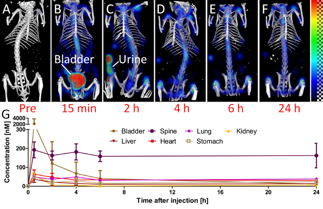
Figure 4. Biodistribution. To assess the biodistribution, the mice are scanned at several time points (A-F). (A) The pre scan, before injection, shows little background signal in the 750 nm channel. (B) 15 min after injection, a considerable amount of the probe is already in the urinary bladder. (C) At the 2 h time point, the mouse had urinated, which results in some fluorescence outside the mouse. At later time points (D-F), the signal appears predominantly at the bones and joints, i.e., at the spine and the knees. (G) The quantified fluorescence concentration is shown for selected organs.

Discussion

We describe and apply a protocol for multimodal µCT-FMT imaging. We use commercially available and widely used FMT and µCT devices^{3,11,15–17,21}. While the protocol requires a specific FMT, the µCT can be replaced by another µCT with similar functionality and comparable scanning parameters, e. g., the field of view should be large enough to cover the mouse bed including the markers.

The FMT has been used for biodistribution analysis without combining it with µCT or MRI²¹, however, the anatomical data is beneficial to increase the reproducibility because the segmentation can be based on the organ boundaries which are visible in the µCT data¹⁰. While integrated µCT-FMT devices have been developed^2,7, these are not commercially available yet. Furthermore, the use of two separate devices allows piping, i.e., the next mouse can be imaged in the µCT while the first mouse is still in the FMT, to increase the throughput.

To reduce the manual workload, we perform automated marker detection and fusion. Furthermore, the mouse shape is automatically segmented and this information significantly improves the fluorescence reconstruction^11,13,22. For quantitative fluorescence reconstruction, absorption and scattering maps are needed^13,23. We derive the scattering map by automated segmentation of the µCT data and assigning known scattering coefficients of several tissue types (lung, bone, skin, fat, and remaining soft tissue)²⁴. Subsequently, we reconstruct an absorption map from the optical raw data which is particularly important for well-perfused organs such as the heart and the liver^13,20.

Scanning several mice at multiple time points quickly results in a large number of data sets to be analyzed. For biodistribution studies, several organs need to be segmented for each µCT-FMT scan. Unfortunately, the segmentations cannot be reused, because the mouse is newly positioned into the mouse bed repeatedly. We use a tool for interactive segmentation, developed at our institute, however, other tools might also be appropriate²⁵. We generate voxel-wise segmentations, because these match better to complex organs than simple shapes such as ellipses and cubes²⁶. Automated whole-animal segmentation would be useful to further reduce the manual workload²⁷, but an interactive segmentation tool would still be required to correct for segmentation errors. Furthermore, automated segmentation tools can hardly anticipate special cases such as pathologies correctly. Since we use native µCT scans, some organs such as the spleen are very difficult to segment even manually. Contrast agents would help, but there are problems with tolerability and it is difficult to maintain a steady contrast agent distribution throughout the longitudinal imaging.

Our phantom study shows that the signal localization is improved when using the shape information for fluorescence reconstruction. In vivo, a similar improvement is evident for the early time point (15 min after injection), when a large amount of the probe is already in the urinary bladder. The hydroxyapatite-binding probe accumulates at bones and joints. It is remarkable how fast this occurs, i.e., the signal is already clearly visible at the spine 15 min after injection. This probably is caused by the low molecular weight of the probe, which enables fast extravasation and diffusion to the target regions. The probe binds covalently to its target hydroxyapatite and the unbound probe is excreted. For the later time points, between 6 h and 24 h after injection, the signal intensity in the spine remains relatively stable, probably, because hardly any light reaches deep into the mouse to bleach the fluorescence. For our study, we used the 750 nm channel, which results in low background fluorescence as evident for the scans acquired before injection. At lower wavelengths, more background signal can be expected²⁸.

In summary, we describe a multimodal imaging protocol for commercially available FMT and µCT devices. We show that the combination provides benefits for fluorescence reconstruction. We illustrate how the biodistribution curves are extracted from the large amount of image data by means of interactive organ segmentation and batch processing. We believe that this standardized workflow can be helpful for drug development and other imaging studies using fluorescently labeled probes.

Materials

List of materials used in this article

Name	Company	Catalog Number	Comments
FMT (Fluorescence molecular tomography) FMT2500 LX	PerkinElmer	FMT2000	Device for fluorescence molecular tomography
µCT (micro computed tomography) Tomoscope Duo	CT Imaging GmbH	Tomoscope Duo	Device for micro computed tomography
Multimodal Mouse Bed	CT Imaging GmbH	Experimental builder	Partially transparent animal holder
IsoFlo (isoflurane, USP)	Abbott	05260-05	Isoflurane Inhalation anesthesia
Small animal anesthesia system	Harvard apparatus	726419	Complete Isoflurane Table-Top System
Chlorophyll-free mouse food	Ssniff	E15051	low chlorophyll / low fluorescence food
OsteoSense 750EX	PerkinElmer	NEV10053EX	Animal FMT contrast agent
Portex Fine Bore Polythene Tubing	Smith medical	800/100/120	Tube for injection catheter
Sterican 30g	BBraun	4656300	Hypodermic needle for catheter
Imeron	Altana pharma	INLA F.1/0203/3.5337.69	CT contrast agent for the phantom inclusions
Agarose	Sigma	90-12-36-6	Agarose for phantom production
TiO2	Applichem	A1900,1000	Titanium oxyde as phantom scattering agent
Trypan blue	Fluka	93595	Trypan blue to adjust phantom light propagation
Cy7	Lumiprobe	15020	Fluorochrome for the phantom inclusions
Lipovenoes 20%	Fresenius Kabi	3094740	Lipid emulsion, scattering agent for FMT contrast agents
Definiens Developer XD Server	Definiens AG	Server XD	Software platform for automated segmentation
Imalytics Preclinical	ExMI/Gremse-IT	Version 2.0.1	Software for image fusion, reconstruction and analysis
NVIDIA Geforce Titan	Asus	GTXTITAN6GD5	High end computer graphics card, 6GB Memory

References

- Hoffman, R. M., Yang, M. Subcellular imaging in the live mouse. Nature Protocols. 1 (2), 775-782 (2006).
- Ale, A., Ermolayev, V., Herzog, E., Cohrs, C., Angelis, M. H., Ntziachristos, V. FMT-XCT: in vivo animal studies with hybrid fluorescence molecular tomography-X-ray computed tomography. Nature Methods. 9 (9), 615-620 (2012).
- Eaton, V. L., Vasquez, K. O., Goings, G. E., Hunter, Z. N., Peterson, J. D., Miller, S. D. Optical tomographic imaging of near infrared imaging agents quantifies disease severity and immunomodulation of experimental autoimmune encephalomyelitis in vivo. Journal of Neuroinflammation. 10 (138), (2013).
- Lederle, W., Arns, S., et al. Failure of annexin-based apoptosis imaging in the assessment of antiangiogenic therapy effects. EJNMMI Research. 1 (26), (2011).
- Ntziachristos, V., Tung, C. -H., Bremer, C., Weissleder, R. Fluorescence molecular tomography resolves protease activity in vivo. Nature Medicine. 8 (7), (2002).
- Hoffman, R. M. The multiple uses of fluorescent proteins to visualize cancer in vivo. Nature Reviews Cancer. 5 (10), 796-806 (2005).
- Schulz, R. B., Ale, A., et al. Hybrid system for simultaneous fluorescence and x-ray computed tomography. IEEE Transactions on Medical Imaging. 29 (2), 465-473 (2010).
- Stuker, F., Baltes, C., et al. Hybrid small animal imaging system combining magnetic resonance imaging with fluorescence tomography using single photon avalanche diode detectors. IEEE Transactions on Medical Imaging. 30 (6), 1265-1273 (2011).
- Leblond, F., Davis, S. C., Valdés, P. A., Pogue, B. W. Preclinical Whole-body Fluorescence Imaging: Review of Instruments, Methods and Applications. Journal of Photochemistry and Photobiology B: Biology. 98 (1), 77-94 (2010).
- Kunjachan, S., Gremse, F., et al. Noninvasive optical imaging of nanomedicine biodistribution. ACS Nano. 7 (1), 252-262 (2013).
- Radrich, K., Ale, A., Ermolayev, V., Ntziachristos, V. Improving limited-projection-angle fluorescence molecular tomography using a co-registered x-ray computed tomography scan. Journal of Biomedical Optics. 17 (12), 126011(2012).
- Freyer, M., Ale, A., Schulz, R. B., Zientkowska, M., Ntziachristos, V., Englmeier, K. -H. Fast automatic segmentation of anatomical structures in x-ray computed tomography images to improve fluorescence molecular tomography reconstruction. Journal of Biomedical Optics. 15 (3), 036006(2010).
- Gremse, F., Theek, B., et al. Absorption Reconstruction Improves Biodistribution Assessment of Fluorescent Nanoprobes Using Hybrid Fluorescence-mediated Tomography. Theranostics. 4 (10), 960-971 (2014).
- Cheong, W. -F., Prahl, S. A., Welch, A. J. A review of the optical properties of biological tissues. IEEE Journal of Quantum Electronics. 26 (12), 2166-2185 (1990).
- Doleschel, D., Mundigl, O., et al. Targeted near-infrared imaging of the erythropoietin receptor in human lung cancer xenografts. Journal of Nuclear Medicine: Official Publication, Society of Nuclear Medicine. 53 (2), 304-311 (2012).
- Al Rawashdeh, W., Arns, S., et al. Optical tomography of MMP-activity allows a sensitive non-invasive characterization of the invasiveness and angiogenesis of SCC-xenografts. Neoplasia. 16 (3), 235-246 (2014).
- Kunjachan, S., Pola, R., et al. Passive versus Active Tumor Targeting Using RGD- and NGR-Modified Polymeric Nanomedicines. Nano Letters. 14 (2), 972-981 (2014).
- Schober, A., Nazari-Jahantigh, M., et al. MicroRNA-126-5p promotes endothelial proliferation and limits atherosclerosis by suppressing Dlk1. Nature Medicine. 20 (4), 368-376 (2014).
- Aikawa, E., Nahrendorf, M., et al. Osteogenesis associates with inflammation in early-stage atherosclerosis evaluated by molecular imaging in vivo. Circulation. 116 (24), 2841-2850 (2007).
- Gremse, F., Höfter, A., Schwen, L., Kiessling, F., Naumann, U. GPU-Accelerated Sparse Matrix-Matrix Multiplication by Iterative Row Merging. SIAM Journal on Scientific Computing. , C54-C71 (2015).
- Vasquez, K. O., Casavant, C., Peterson, J. D. Quantitative Whole Body Biodistribution of Fluorescent-Labeled Agents by Non-Invasive Tomographic Imaging. PLoS ONE. 6 (6), e20594(2011).
- Theek, B., Gremse, F., et al. Characterizing EPR-mediated passive drug targeting using contrast-enhanced functional ultrasound imaging. Journal of Controlled Release. 182 (1), 83-89 (2014).
- Hyde, D., Schulz, R., Brooks, D., Miller, E., Ntziachristos, V. Performance dependence of hybrid x-ray computed tomography/fluorescence molecular tomography on the optical forward problem. Journal of the Optical Society of America. A, Optics, Image Science, and Vision. 26 (4), 919-923 (2009).
- Jacques, S. L. Optical properties of biological tissues: a review. Physics in Medicine and Biology. 58 (11), R37(2013).
- Loening, A. M., Gambhir, S. S. AMIDE: a free software tool for multimodality medical image analysis. Molecular Imaging. 2 (3), 131-137 (2003).
- Gremse, F., Schulz, V. Qualitative and Quantitative Data Analysis. Small Animal Imaging. , 363-378 (2011).
- Baiker, M., Milles, J., et al. Atlas-based whole-body segmentation of mice from low-contrast Micro-CT data. Medical Image Analysis. 14 (6), 723-737 (2010).
- Sevick-Muraca, E. M., Rasmussen, J. C. Molecular imaging with optics: primer and case for near-infrared fluorescence techniques in personalized medicine. Journal of Biomedical Optics. 13 (4), 041303(2008).
Reprints and Permissions