Probing Structural and Dynamic Properties of Trafficking Subcellular Nanostructures by Spatiotemporal Fluctuation Spectroscopy

Summary

Imaging-derived mean square displacement (iMSD) analysis is applied to macropinosomes to highlight their intrinsic time-evolving nature in terms of structural and dynamic properties. Macropinosomes are then compared to insulin secretory granules (ISGs) as a reference for subcellular structures with time-invariant average structural/dynamic properties.

Abstract

Imaging-derived mean square displacement (iMSD) is used to address the structural and dynamic properties of subcellular nanostructures, such as vesicles involved in the endo/exocytotic trafficking of solutes and biomolecules. iMSD relies on standard time-lapse imaging, is compatible with any optical setup, and does not need to dwell on single objects to extract trajectories. From each iMSD trace, a unique triplet of average structural and dynamic parameters (i.e., size, local diffusivity, anomalous coefficient) is calculated and combined to build the "iMSD signature" of the nanostructure under study.

The potency of this approach is proved here with the exemplary case of macropinosomes. These vesicles evolve in time, changing their average size, number, and dynamic properties passing from early to late stages of intracellular trafficking. As a control, insulin secretory granules (ISGs) are used as a reference for subcellular structures that live in a stationary state in which the average structural and dynamic properties of the whole population of objects are invariant in time. The iMSD analysis highlights these peculiar features quantitatively and paves the way to similar applications at the sub-cellular level, both in the physiological and pathological states.

Introduction

Subcellular nanostructures (e.g., endocytic/secretory vesicles, organelles) play a pivotal role in cell-signaling regulation¹. Proper tuning of their structural (e.g., size) and/or dynamic (e.g., diffusivity) characteristics determines how the cell responds to internal or external stimuli^2,3,4. Based on this evidence, it is not surprising that alterations of these characteristics are found in many pathological conditions. Examples encompass the role of misregulated endocytosis in cancer^2,3, the structural and dynamic alterations found at the level of ISGs in β-cells exposed to Type-2 Diabetes conditions⁵, the misregulation of lysosomal structural and transport properties in globoid-cell leukodystrophy or galactosylceramide lipidosis⁶, and dysfunctionalities in the endo-lysosomal pathway in neurodegenerative disorders (e.g., Alzheimer's disease)⁷.

In this context, researchers have recently proved that the performance of standard optical microscopy methods can be enhanced by properly tuning spatial and temporal sampling resolution⁸. This, in turn, may provide further insight into biological processes of relevance. In practice, this is made possible by an algorithm of spatiotemporal fluctuation analysis, which simultaneously extracts the average structural and dynamic properties of diffusing objects directly from the standard stack of optical microscopy images without any need for preliminary knowledge on the biological object of interest and extraction of single-object trajectories. All this information is enclosed in a single output of the method: an iMSD trace⁹ (details on the iMSD trace derivation and analysis are given in Supplemental File 1).

The resulting experimental protocol consists of a few steps. First, imaging of the region of interest is performed at high temporal resolution. Then, average spatial-temporal correlation functions are calculated from the stack of images. Finally, by Gaussian fitting of the series of correlation functions, the average 'diffusion law' is obtained directly from imaging and analyzed to recognize the object diffusion mode. The potential of the method was already proved for a variety of biological objects, ranging from molecules to nanoparticles and even entire subcellular organelles/structures^{9,10,11,12,13,14,15}.

This paper reports iMSD application to macropinosomes to highlight their intrinsic, irreversible time-evolving nature in terms of their average (i.e., at the whole population level) structural and dynamic properties. Further, these endocytic vesicles are compared to ISGs as a reference for subcellular structures in a 'stationary state', i.e., a state in which the average structural/dynamic properties of the whole population of granules remain constant at any time point. Macropinocytosis defines a series of events initiated by the extensive reorganization (or ruffling) of the plasma membrane to form an external macropinocytic structure that is then internalized¹⁶. The formed early-stage macropinosomes are very similar to phagosomes. At the same time, they can be distinguished from other forms of endocytic vesicles owing to their characteristic large size, morphological heterogeneity, and lack of protein-coat structures.

Biochemical assays revealed that, upon internalization, macropinosomes progressively get enriched with protein markers of other endocytic pathways, in turn, suggesting that their identities are continuously changing during trafficking¹⁷. Using antibodies against known markers of the endosomal pathway, it was demonstrated that macropinosomes progressively adopt classical endosomal features: they diminish in size, develop into late endocytic structures (e.g., lysosomes), or eventually lose their identity via membrane-mediated retrieval of specific molecular markers (e.g., sorting nexins)^18,19. The overall scenario is that every single macropinosome within the cell irreversibly changes its structural and dynamic (as well as molecular) identity during trafficking from the plasma membrane to its final intracellular fate. As a result, the structural/dynamic/molecular properties of the whole population of macropinosomes are also changing along the same temporal path. Being intrinsically sensitive to the average properties of the whole population of observed objects, the iMSD method quantitatively depicts the 'evolving nature' by the quantification of key average parameters, i.e., the local diffusivity and anomalous coefficient (dynamic properties) and the average size of the macropinosomes (structural property) at any stage of their intracellular trafficking.

For comparison, similar measurements were performed on a well-known intracellular membrane-enclosed structure, the ISG, in a model of β-cells. Like macropinosomes, the regulation of the structural and dynamic properties of ISGs, from their genesis at the Trans Golgi Network (TGN) to their exocytosis at the plasma membrane, is pivotal to the proper execution of ISG function²⁰. However, unlike macropinosomes, ISGs live in a 'stationary state' in which, at any time, all the functional/structural/molecular stages of ISG lifespan are simultaneously present within the cell, and each is represented by a specific subpopulation of ISGs. This means that although every single granule irreversibly evolves from biogenesis to secretion, the average structural/dynamic properties of the whole population of granules is expected to remain constant at any time point (unless the stationary state conditions are changed, for instance, by external stimuli such as glucose, cholesterol, and cytokines¹³). This is confirmed by iMSD analysis.

Protocol

1. Sample preparation

1. Before the microscopy experiment, subculture cells in dishes suited for microscopy applications.
   1. Wash a 10 cm tissue-culture-treated dish of confluent HeLa or INS 1E (insulinoma β-cell-like) cells twice with 0.01 M 1x PBS, add 1 mL of 0.05% trypsin-EDTA (1x), and place it in a 37 °C, humidified, 5% CO₂ incubator for 5 min.
   2. Resuspend the detached cells by adding 9 mL of complete DMEM (for HeLa cells) or RPMI 1640 (for INS-1E cells) medium, and collect the final 10 mL in centrifuge tubes.
   3. Seed approximately 2 × 10⁵ cells in each 35 mm x 10 mm dish in a final volume of 1 mL of the medium. Incubate the cells for 24 h at 37 °C and 5% CO₂.
2. To fluorescently label lysosomes, use LysoTracker Red DND-99.
   1. Dilute the stock solution in 1 mL of prewarmed medium to a final dye concentration of 70 nM.
   2. Replace the medium from the dish with fresh LysoTracker-containing medium. Incubate the cells in LysoTracker-containing medium for 20 min at 37 °C in a 5% CO₂ atmosphere, and wash them twice with fresh medium before the experiment.
   3. To fluorescently label macropinosomes, use 70-kDa fluorescein isothiocyanate-dextran. Wash the subcultured cells three times with 0.01 M 1x phosphate-buffered saline (PBS), replace with dextran-containing medium (1 mg/mL), and incubate at 37 °C for 30 min. Before proceeding with the microscopy experiment, wash the cells three times with fresh medium.
   4. To fluorescently label ISGs in INS-1E cells, transfect the cells using transfection reagent (see the Table of Materials) and C-peptide-enhanced green fluorescent protein (EGFP) plasmid¹³ according to the manufacturer's protocol, and incubate at 37 °C for 24 h in a 5% CO₂ atmosphere before the experiment.

2. Data Acquisition

1. To let the microscope equilibrate at the desired temperature and atmosphere, turn on the microscope incubator-controlling system at least 2 h before the experiment.
   NOTE: Each acquisition is a time-lapse series.
2. Acquire the images using an inverted confocal microscope equipped with a 60x, 1.2 Numerical Aperture (NA) water-immersion objective.
3. Use a 488 nm Argon laser for excitation of EGFP (transfected cells) and fluorescein-labeled macropinosomes. Collect the fluorescence emission between 500 and 600 nm using a standard photomultiplier tube detector.
4. Use a 543 nm HeNe laser to excite Lysotracker and collect its fluorescence emission between 555 and 655 nm.
5. Set the diameter of the detection pinhole to the size of 1 Airy. For each acquisition, collect a series of 1000 sequential frames. Set the pixel-dwell time to 2 µs/pixel for a frame time of 129 ms.
   ​NOTE: Each frame consisted of 256 x 256 pixels (16 bit/pixel) with a physical dimension of 69 nm/pixel, corresponding approximately to an area of 17 µm x 17 µm.

3. iMSD calculation

NOTE: To properly execute the calculation, use software capable of numeric calculation and script programming. The specific script (i.e., for the 'iMSD.m' script file, see Supporting File 1) must be present in the same directory containing the image series to be processed. Each image of the series must be saved as a distinct '.tif' file.

1. To properly initialize the instrumental parameters used for the acquisitions, open iMSD.m with the software text editor and modify its first section as follows.
   1. Set N as the number of frames in the time series (e.g., 1000 in this protocol).
   2. Set px_size: pixel size, expressed in µm (e.g., 0,069 in this protocol).
   3. Set f: temporal resolution of each frame, expressed in seconds (e.g., 0,129 in this protocol).
   4. Set Filter: binary input for background correction, set the value to '0' to process raw images, or set the value to '1' to perform a threshold-based background subtraction.
   5. Set av_toll: threshold for background correction; any pixel with intensity lower than this value will be set as 0 if Filter=1.
   6. Set bit as the integer number determining the intensity sampling (e.g., 8 bit, 16 bit).
2. Save and run the edited iMSD.m script file.
3. Check the script execution.
   NOTE: The calculation processing status can be checked on the command window; if any fatal problem occurs, the process will be interrupted, and a warning message will be displayed to show the error type and the related line code. Otherwise, follow steps 3.3.1-3.3.3.
   1. Import the image stack and subtract the background (if required).
   2. Calculate the spatiotemporal correlation function G(ξ,η,τ) using the Fourier method.
   3. Fit the spatiotemporal correlation function with a 2D Gaussian function.
      NOTE: At the end of the process, the output values of the σ²(τ) fitting procedures will be shown in the command window: averages, error, and corresponding goodness (R²) of fitting are reported.
4. Check the graphical output.
   NOTE: The iMSD curve and the corresponding fitting curves are shown in three separate panels, each for a different type of fitting equation used: Brownian diffusion, anomalous diffusion, or confined diffusion. For each curve, the R² value is reported in the graph legend.
5. Check the text output.
   NOTE: At the end of the process, an '.xls' file is created with the same name of the original time-lapse '.tif' file. The first sheet contains the values of ξ, η, τ, and σ² calculated for each time-delay. The input parameters and principal calculated output values are reported in the second sheet, i.e., diffusion coefficient, anomalous coefficient, and y-axis σ²₀ intercept.

Results

The general workflow of the method is presented in Figure 1. It recapitulates the main steps presented in the protocol section, from sample preparation (Figure 1A) to time-lapse imaging of intracellular nanostructures (Figure 1B), fluctuation analysis for the calculation of the series of spatiotemporal correlation functions (Figure 1C), and fitting for the derivation of the average structural/dynamic properties of the object under study (Figure 1D).

A critical parameter is the time resolution adopted for imaging the subcellular object of interest. This experimental value will set the time threshold at which the minimum average displacement of the objects of interest will be measured. However, the preferred condition is setting a time resolution of imaging at which the object of interest appears 'immobile' within the captured frame, i.e., it displays a characteristic size that, on average, is not deformed due to the imaging speed. This is technically possible if the object of interest is a membrane-enclosed subcellular structure or organelle (as in this case). Typically, subcellular structures exhibit local diffusion coefficients (D, µm²/s, see Table 1) that are several orders of magnitude lower than those of isolated single molecules in the cytoplasm (e.g., GFP²¹). Validation can be performed by artificially immobilizing the organelle of interest (e.g., by chemical fixation). Indeed, this condition can serve as a reference to determine the actual organelle size under the experimental conditions used (e.g., excitation wavelength, pixel size, objective).

Here, although lysosomes were used as test organelles for this procedure, the results are valid independently from the target structure. Figure 2A shows an image of a fixed (i.e., immobile) lysosome along with an acquisition performed on live cells at the appropriate temporal resolution (i.e., typically below 100 ms/frame; e.g., 65 ms/frame in the example in Figure 2B) and an acquisition performed intentionally at very low temporal resolution (e.g., 10 s/frame in the example in Figure 2C). For each condition, the size of the diffusing object is extracted as follows: i) an intensity profile of the spot is derived by the line tool in ImageJ software; ii) the intensity profile is plotted and interpolated by a Gaussian function to calculate the full width at half maximum (FWHM) value that, in turn, is used as an estimate of the spot diameter (Figure 2D). As expected and shown in the plot of Figure 2E, the acquisition at very high temporal resolution (i.e., 65 ms/frame) yields an average size of the structure close to that obtained in the fixed sample, either by using the standard tool described above or by extracting the iMSD y-axis intercept. Instead, the acquisition at slow speed yields an increase in the apparent size of the structure, owing to the natural structure dynamics during imaging. Under suboptimal experimental conditions, the structural/dynamic information extracted does not faithfully reflect the intrinsic properties of the object under study.

Once the main experimental parameters are selected, datasets can be produced for the target intracellular structures. For macropinosomes, after 20 min of incubation of the cells with 70 kDa dextrans, time series of the labeled intracellular structures were acquired at different time points after treatment, from 30 min up to approximately 180 min. Interestingly, a gradual change in the structural and dynamic properties of macropinosomes is detected during trafficking (Figure 3; distributions of σ₀², D_m, α, and N for macropinosomes are reported in the plots on the left). While no obvious changes in the local diffusivity (D_m) of macropinosomes are detected during trafficking, both the characteristic size (σ₀²) and overall mode of motion (α) evolve in time.

Of particular note, a decrease in the average size of the macropinosomes is observed during trafficking (Figure 3A, left), together with a concomitant increase in the subdiffusive nature of their motion (i.e., denoted as a decrease in α values, Figure 3C, left panel). Additionally, the number of macropinosomes was extracted from each acquisition: the results, reported in Figure 3D, left panel, clearly reveal an increase in the number of macropinosomes in time. All these results are in good agreement with the expectations because dextran-labeled macropinosomes are supposed to originate as isolated, large membrane-enclosed vesicles at the plasma membrane (that are also competent for movement along cytoskeletal components) but are supposed to gradually communicate with the endo-lysosomal pathway made up of a large population of smaller and randomly diffusing structures.

As anticipated above, the results for macropinosomes are in contrast to similar measurements performed on ISGs (Figure 3, right column). Insulin granules do not show a time-evolving trend of the iMSD-derived structural/dynamic parameters (and their average number within the cell) in the same time window observed for macropinosomes. Moreover, the characteristic values of σ₀², D_m, and α are quite different from those of lysosomes, used again as a reference. This result confirms the idea, as anticipated above, that granules are probed in a 'stationary state' in which, at any time, the average structural/dynamic properties of the whole population of ISGs are unchanged (i.e., they remain constant, unless the stationary-state conditions change, for instance, due to external stimuli).

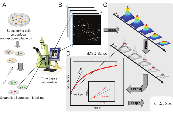
Figure 1: Experimental workflow. (A) Cells were plated 24 h (48 h for transfection experiments) before confocal experiments onto cell dishes suited for microscopic applications. Cells were then suitably treated according to the labeling method (see protocol) to stain the cytoplasmic organelle of interest. (B) A typical confocal acquisition consists of a stack of images (time-lapse) of a cytoplasmic portion of a living cell, describing the time-evolution of labeled organelle dynamics. (C) Time-lapse movie is analyzed with a custom-made Matlab script, first calculating spatiotemporal image correlation function and Gaussian fitting to plot iMSD curves (D) and related extracted fitting parameters describing structural dynamics parameters of imaged organelles. Abbreviations: iMSD = imaging-derived mean square displacement; STICS = spatiotemporal image correlation spectroscopy; α = anomalous diffusion coefficient; D_m = local diffusivity; σ²(τ) = variance. Please click here to view a larger version of this figure.

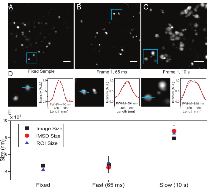
Figure 2: Proper experimental parameters. (A) Exemplary image of stained lysosomes in a fixed sample. Scale bar = 2 µm. (B) The first frame of a stack of images of stained lysosomes in a living cell, acquired with the appropriate parameters. Temporal resolution: 65 ms/frame. Scale bar = 2 µm. (C) The first frame of a stack of images of stained lysosomes in a living cell, acquired at low speed: artifactual deformation of the apparent lysosome size due to organelle motion during imaging is visible. Temporal resolution: 10 s/frame. Scale bar = 2 µm. (D) Example of size calculation for imaged lysosomes in a blue ROI of (A), (B), and (C). The intensity profile along the blue line was fitted with a Gaussian function to retrieve the FWHM, i.e., an estimate of spot size. FWHM values are reported for each fitting. (E) Graphical representation of size values obtained by image analysis described in panel (D) for all imaged lysosomes (black square, mean value, and standard deviation), for lysosomes enclosed within the blue ROI (blue triangle), and retrieved by iMSD analysis (red circle). This figure is from ²². Abbreviations: ROI = region of interest; FWHM = full-width at half-maximum; iMSD = imaging-derived mean square displacement. Please click here to view a larger version of this figure.

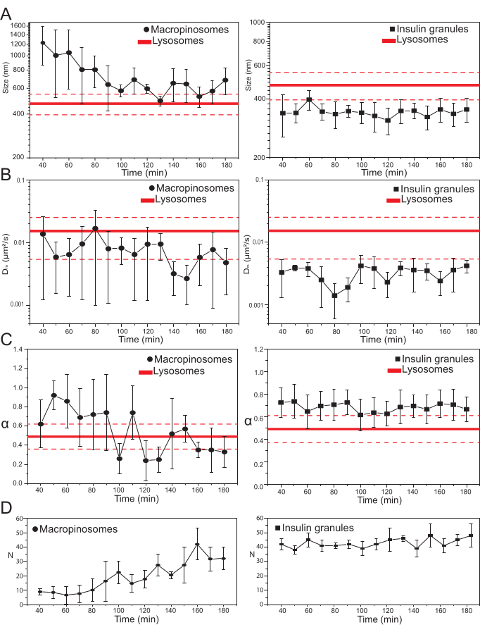
Figure 3: Temporal evolution of labeled organelles. (A) Plots of iMSD-extracted size values vs. time progression of subsequent acquisitions represented as a mean of measured values in acquisitions performed on a 10-min time window. On the left, progressive reduction in the average size of macropinosomes (black circles) and on the right, the time-invariant size of insulin secretory granules (black squares) compared to lysosomes, represented as average size value (thicker red line) ± standard deviation (dashed red lines). (B) and (C) Time progression of D_m and α coefficients for macropinosomes (left) and insulin granules (right) extracted by iMSD analysis. (D) Time-evolution of numbers of labeled macropinosomes and insulin granules measured in the first frame of each acquired time-lapse movie. Abbreviations: iMSD = imaging-derived mean square displacement; α = anomalous diffusion coefficient; D_m = local diffusivity, N = number. Please click here to view a larger version of this figure.

Organelle		Labelling		Cell Line	Size (nm)	Dm ( × 10-3 μm2/s)	α	N	Ref.
Early Endosome (EE)		CellLight Early Endosome GFP		HeLa	395±74	3.0±2.4	1.02±0.20	40	10
Late Endosome (LE)		CellLight Late Endosome GFP		HeLa	693±102	15.4±10.6	0.57±0.16	58	10
Lysosome (LY)		LysoTracker DND-99		HeLa	471±76	15.3±9.0	0.49±0.13	143	10, 14
Caveola (CAV)		Caveolin-EGFP		HeLa	405±49	3.1±1.8	1.00±0.22	15	10
Clathrin Coated Vescicle (CCV)		Transferrin-Alexa 488		HeLa	513±62	16.2±9.9	0.48±0.17	33	10
Insulin Granule (IG)		C-peptide-EGFP		INS-1E	335±56	3.0±1.7	0.70±0.14	107	11
Early Macropinosome (EMCR)		Fluorescein-Dextran 70 kDa		HeLa	979±423	8.3±9	0.79±0.27	36	10
Intermediate Macropinosome (IMCR)		Fluorescein-Dextran 70 kDa		HeLa	702±180	13.7±19.9	0.60±0.38	29	10
Late Macropinosome (LMCR)		Fluorescein-Dextran 70 kDa		HeLa	592±127	5.8±4.7	0.39±0.21	21	10

Table 1: Structural and dynamic iMSD-extracted parameters. The table shows the values of size, D_m, and α coefficient measured for different organelles, specifying labeling strategies, the cell line used, and the number of analyzed acquisitions. Values are reported as mean ± standard deviation. Abbreviations: iMSD = imaging-derived mean square displacement; α = anomalous diffusion coefficient; D_m = local diffusivity, N = number; GFP = green fluorescent protein; EGFP = enhanced green fluorescent protein.

Supplemental File 1: Details on the iMSD trace derivation and analysis. Please click here to download this File.

Supporting File 1: Please click here to download this File.

Discussion

The properties and advantages of iMSD are evident when compared to the techniques available to retrieve analogous information. For structural information, the preferred choice is transmission electron microscopy (TEM) analysis. By this method, ultrastructural details at molecular resolution and even beyond can be retrieved, even for subcellular nanostructures. Nevertheless, the peculiar spatial resolution of TEM is achieved at the expense of the information in the temporal dimension, which is of interest here. To compensate for this, the recent advances in live-cell imaging technologies are of particular interest. These include new fluorescent markers with increased performances (e.g., brightness and photostability), optimized labeling procedures, and more sensitive detectors. In addition, analytical tools are available to address both structural (e.g., 'size' by phasor-based analysis of local image correlation spectroscopy, PLICS²³, aggregation/oligomerization by Number&Brightness analysis²⁴) and dynamic (e.g., diffusion law by single-particle tracking, i.e., (SPT)^25,26,27,28) parameters on the subcellular scale. The SPT method affords direct access to the object trajectory and its MSD. However, the disadvantage is the need for a low density of the probe and very bright labels and many single-object trajectories to be measured to satisfy statistical criteria. With respect to the temporal resolution of the measurement, inorganic, photostable probes (e.g., quantum dots or metal nanoparticles) can increase SPT performance but at the expense of complex production and labeling procedures.

Compared to these standards, the iMSD method described here shows some key advantages. First, this approach can be used in conjunction with relatively dim fluorescent tags, such as genetically encoded fluorescent proteins (e.g., the application to ISGs). Thus, compared to SPT, a higher temporal resolution is achieved (using the same label) due to the lower amount of photons required⁸. Second, the iMSD method is limited only by the temporal resolution but not diffraction. In fact, despite the diffraction-limited optical setup used, average molecular displacements even below the diffraction limit can be measured, as already demonstrated for molecular flows by using STICS²⁹. The actual resolution in the measurement of displacements depends on how accurately (in terms of signal to noise) the correlation function can be measured, thus explaining why it is not limited by diffraction. Thus, it appears clear that the minimum displacement that can be measured depends on the diffusivity of the object of interest and the temporal resolution of the imaging setup.

In this regard, it is important to consider that application to subcellular nanostructures, such as macropinosomes or insulin granules, with a laser scanning microscope is optimal: the scanning speed available is significantly higher than the dynamics of the object of interest. In such a case, the movement of the objects during the acquisition is negligible, and the correlation function can be approximated by a Gaussian function. Finally, the iMSD approach can be easily applied to a wide range of commercial optical microscopy setups based on raster scan or wide-field camera-based imaging, with no need for system calibration (required only if an accurate estimate of particle size needs to be achieved). An important parameter for the method to work is proper spatial sampling. As a general rule, to reach satisfactory convergence of the fitting algorithm, the minimum size of the region of interest for imaging should be at least 3 times larger than the maximum displacement of interest.

In conclusion, the iMSD method requires only a microscope equipped for fast acquisition. The structure of interest can be tagged to any genetically encoded or organic fluorophore, thus enabling multichannel imaging. It is envisioned that cross-iMSD analysis will be used in the near future to select subpopulations of subcellular nanostructures and reveal their interactions and co-diffusion within the cell, the latter being a hot topic in cellular biophysics. If any detail is lost by iMSD analysis, this is certainly related to the large amount of molecular information within dynamic subcellular nanostructures. Such information is inevitably averaged out during the measurement due to poor temporal resolution. Theoretically, however, there is no technical limit due to the possibility to retrieve molecular information, provided that sufficient acquisition speeds can be achieved⁸. Due to the continuous improvements in detector speed/sensitivity and imaging technologies, it is envisioned that information about the whole subcellular compartment and its molecular constituents will be extracted from a single dataset.

Materials

List of materials used in this article

Name	Company	Catalog Number	Comments
100x Penicillin-Streptomycin-Glutamine	Gibco	10378-016	Cell medium supplement
C-peptide-EGFP			Plasmid
DMEM High Glucose	Gibco	31053028	Cell medium (HeLa)
FBS	Gibco	10082147	Cell medium supplement
Fluorescein isothiocyanate-dextran 70 kDa	Sigma Aldrich	46945-100MG-F	Reagent
HeLa	ATCC	CCL-61	Cell Line
Lipofectamine 2000	TermoFisher	11668019	Trasfection reagent
Lysotracker Red DND-99	Gibco	L7528	Reagent
Matlab	MathWork		Software
Microscope-suitable cell dishes	Willco	GWSt-3522	Petri dishes
Olympus FV1000	Olympus Japan		Confocal microscope
RPMI 1640	Gibco	11835063	Cell medium (INS-1E)

References

- Murphy, J. E., Padilla, B. E., Hasdemir, B., Cottrell, G. S., Bunnett, N. W. Endosomes: a legitimate platform for the signaling train. Proceedings of the National Academy of Sciences of the United States of America. 106 (42), 17615-17622 (2009).
- Mosesson, Y., Mills, G. B., Yarden, Y. Derailed endocytosis: an emerging feature of cancer. Nature Reviews Cancer. 8 (11), 835-850 (2008).
- Mellman, I., Yarden, Y. Endocytosis and cancer. Cold Spring Harbor Perspectives in Biology. 5 (12), 016949(2013).
- Di Fiore, P. P. Endocytosis, signaling and cancer, much more than meets the eye. Preface. Molecular Oncology. 3 (4), 273-279 (2009).
- Bogan, J. S., Xu, Y., Hao, M. Cholesterol accumulation increases insulin granule size and impairs membrane trafficking. Traffic. 13 (11), 1466-1480 (2012).
- Ballabio, A., Gieselmann, V. Lysosomal disorders: From storage to cellular damage. Biochimica et Biophysica Acta. 1793 (4), 684-696 (2009).
- Hu, Y. -B., Dammer, E. B., Ren, R. -J., Wang, G. The endosomal-lysosomal system: from acidification and cargo sorting to neurodegeneration. Translational Neurodegeneration. 4, 18(2015).
- Di Rienzo, C., Gratton, E., Beltram, F., Cardarelli, F. Spatiotemporal fluctuation analysis: a powerful tool for the future nanoscopy of molecular processes. Biophysical Journal. 111 (4), 679-685 (2016).
- Di Rienzo, C., Gratton, E., Beltram, F., Cardarelli, F. Fast spatiotemporal correlation spectroscopy to determine protein lateral diffusion laws in live cell membranes. Proceedings of the National Academy of Sciences of the United States of America. 110 (30), 12307-12312 (2013).
- Di Rienzo, C., Gratton, E., Beltram, F., Cardarelli, F. From fast fluorescence imaging to molecular diffusion law on live cell membranes in a commercial microscope. Journal of Visualized Experiments: JoVE. (92), e51994(2014).
- Digiacomo, L., et al. Dynamic fingerprinting of sub-cellular nanostructures by image mean square displacement analysis. Scientific Reports. 7 (1), 14836(2017).
- Durso, W., et al. Lysosome dynamic properties during neuronal stem cell differentiation studied by spatiotemporal fluctuation spectroscopy and organelle tracking. International Journal of Molecular Sciences. 21 (9), 3397(2020).
- Ferri, G., et al. Insulin secretory granules labelled with phogrin-fluorescent proteins show alterations in size, mobility and responsiveness to glucose stimulation in living β-cells. Scientific Reports. 9 (1), 2890(2019).
- Durso, W., D'Autilia, F., Amodeo, R., Marchetti, L., Cardarelli, F. Probing labeling-induced lysosome alterations in living cells by imaging-derived mean squared displacement analysis. Biochemical and Biophysical Research Communications. 503 (4), 2704-2709 (2018).
- Digiacomo, L., Digman, M. A., Gratton, E., Caracciolo, G. Development of an image Mean Square Displacement (iMSD)-based method as a novel approach to study the intracellular trafficking of nanoparticles. Acta Biomaterialia. 42, 189-198 (2016).
- Swanson, J. A., Watts, C. Macropinocytosis. Trends in Cell Biology. 5 (11), 424-428 (1995).
- Jones, A. T. Macropinocytosis: searching for an endocytic identity and role in the uptake of cell penetrating peptides. Journal of Cellular and Molecular Medicine. 11 (4), 670-684 (2007).
- Falcone, S., et al. Macropinocytosis: regulated coordination of endocytic and exocytic membrane traffic events. Journal of Cell Science. 119, Pt 22 4758-4769 (2006).
- Kerr, M. C., et al. Visualisation of macropinosome maturation by the recruitment of sorting nexins. Journal of Cell Science. 119, Pt 19 3967-3980 (2006).
- Rorsman, P., Renstrom, E. Insulin granule dynamics in pancreatic beta cells. Diabetologia. 46 (8), 1029-1045 (2003).
- Di Rienzo, C., Piazza, V., Gratton, E., Beltram, F., Cardarelli, F. Probing short-range protein Brownian motion in the cytoplasm of living cells. Nature Communications. 5 (1), 5891(2014).
- Ferri, G., et al. Time-lapse confocal imaging datasets to assess structural and dynamic properties of subcellular nanostructures. Scientific Data. 5 (1), 180191(2018).
- Scipioni, L., Gratton, E., Diaspro, A., Lanzanò, L. Phasor analysis of local ICS detects heterogeneity in size and number of intracellular vesicles. Biophysical Journal. 111 (3), 619-629 (2016).
- Digman, M. A., Dalal, R., Horwitz, A. F., Gratton, E. Mapping the number of molecules and brightness in the laser scanning microscope. Biophysical Journal. 94 (6), 2320-2332 (2008).
- Li, C. H., Bai, L., Li, D. D., Xia, S., Xu, T. Dynamic tracking and mobility analysis of single GLUT4 storage vesicle in live 3T3-L1 cells. Cell Research. 14 (6), 480-486 (2004).
- Donovan, K. W., Bretscher, A. Tracking individual secretory vesicles during exocytosis reveals an ordered and regulated process. Journal of Cell Biology. 210 (2), 181-189 (2015).
- Westphal, V., et al. Video-rate far-field optical nanoscopy dissects synaptic vesicle movement. Science. 320 (5873), 246-249 (2008).
- Tabei, S. M. A., et al. Intracellular transport of insulin granules is a subordinated random walk. Proceedings of the National Academy of Sciences of the United States of America. 110 (13), 4911-4916 (2013).
- Hebert, B., Costantino, S., Wiseman, P. W. Spatiotemporal image correlation spectroscopy (STICS) theory, verification, and application to protein velocity mapping in living CHO cells. Biophysical Journal. 88 (5), 3601-3614 (2005).
Reprints and Permissions