Surrogate Model Development for Digital Experiments in Welding

Summary

This protocol outlines a general workflow for constructing an artificial neural network for welding simulation using datasets generated automatically through Python scripts with macro functions. The workflow is validated against a benchmark case involving single-pass, straight-line welding. The surrogate model's predictive accuracy shows a strong agreement with finite element simulations.

Abstract

The manufacturing industry heavily relies on welding processes to join materials, forming integral components across various sectors. Many aspects will influence the quality of the weld and finally affect the structure integrity of the weldment. Welding-induced residual stress, a consequence of the thermal cycling inherent in these processes, significantly impacts the structural integrity and performance of fabricated components. Understanding and predicting this residual stress is crucial for enhancing the reliability and durability of welded structures. However, quickly assessing a welding setup in digital experiments presents significant challenges, as a traditional simulation may be time-consuming. This research outlines the application of a workflow to construct an artificial neural network-based surrogate model to predict welding-induced residual stress. The model is built using data automatically generated from finite element simulations through Python scripts based on macro functions. Unlike traditional methods that rely on manual preprocessing and finite element simulations, this approach significantly reduces the time and effort required for simulation setup and data extraction, enhancing overall efficiency. By ensuring that all simulation steps are performed consistently through macro functions, the method eliminates human-induced variability, leading to improved reproducibility. Furthermore, the automation of data generation makes it possible to create extensive datasets necessary for training machine learning models, overcoming the limitations of labor-intensive traditional techniques. The workflow contains four main steps: build a standard weld finite element simulation and validate the finite element simulation results against experimental data; develop scripts for large dataset generation using a macro function that records the preprocessing and postprocessing steps of the finite element simulation; use the scripts to generate the required data; develop surrogate models and test their performance. The artificial neural network demonstrated high accuracy in predicting stress levels, closely aligning with simulation results on the test dataset and a relative root mean square error of 0.0024.

Introduction

When performing a digital experiment for welding practice, residual stress is a key outcome, as it is a critical aspect of structural integrity assessment. Welding-induced residual stress is caused by the combination of high temperatures, rapid cooling, and the resulting non-uniform thermal gradients and mechanical constraints during the welding process¹. The metal maintains stress even after the internal temperature gradient subsides as a result of plastic deformation and external clamping. Residual stress can have a significant influence on the behavior and performance of components, particularly those that are subject to cyclic loading or high stress. It can cause cracking^2,3 and affect the overall fatigue life⁴.

In order to improve the reliability of the characterization of welding residual stress distribution, groups like the European Network on Neutron Techniques Standardization for Structural Integrity (NeT)⁵ held a series of round-robin activities to conduct experiments and implemented Finite element (FE) simulations for different welding scenarios, such as single weld bead-on-plate weld⁶ and multiple-pass slot weld^7,8. Different techniques of experimental measurement are used to quantify the weld-induced residual stress, including Neutron diffraction⁹, contour method, X-ray diffraction, deep hole drilling¹⁰, and incremental center hole drilling¹¹. In addition to experimental measurement, finite element simulation is also used to reconstruct the residual stress field. Gilles et al.¹² used the surface heat source model in the finite element model to simulate bead-on-plate weld; they also conducted sensitivity analyses of mesh design and heat source models. Shan et al.¹³conducted a thermal-mechanical sequentially coupled analysis to predict after-weld residual stress distribution; they used a moving heat source model with an element birth-or-death technique to characterize heat flux distribution. Bate et al.¹⁴described how to do heat source model calibration on a simplified 2D model of the specimen to ensure the reliability of the welding thermal analysis. Coules et al.¹⁵ presented a method for reconstructing residual stress fields in an incompatible region by combining measurements from several nearby regions. The paper highlighted the potential of this method for improving the accuracy of residual stress measurements, particularly in situations where measurements in the desired region are not possible. Bouchard⁶put forward a benchmark for bead-on-plate weld simulation and offered a definition of thermal and residual stress performance targets that could be used for weld simulation approach evaluation. Smith et al.¹⁶ reviewed the different weld simulation modeling methods and presented sensitivity analyses of many welding simulation modeling parameters, including mesh design, heat source characteristics, heat input, and constitutive model. The accuracy of simulation results largely depends on the analysts' assumptions and simplifications. Additionally, some details for simulation settings in the previously published papers are often neglected, which makes it difficult to replicate simulations.

In addition to FE simulation, a series of machine learning algorithms have been implemented for stress prediction, which includes fuzzy neural network¹⁷, support vector regression^18,19,20 adaptive neuro-fuzzy network^21,22 artificial neural network²³. The use of pretrained machine learning algorithms significantly reduces the time required for stress prediction compared to finite element analysis. Instead of modeling based on mathematics and physics and then solving differential equations, surrogate model development directly builds relationships between inputs and outputs. Nevertheless, this data-driven methodology conventionally demands a substantial volume of training data. Despite this requisite, there is presently a dearth of published research explaining in detail the process of automating the generation of such data.

The overall goal here is to develop a streamlined workflow for automating data generation from finite element simulations and utilizing the generated data to train machine learning-based surrogate models, such as Artificial Neural Networks (ANNs), for predicting critical outcomes in complex physical processes. Figure 1 presents a high-level flow chart that summarizes the steps in the workflow. This work presents all the settings to conduct a thermal-mechanical welding simulation in Abaqus. By utilizing the macro recording function, all the operations for pre-processing and post-processing in FE simulation are recorded into scripts, thereby automating the data generation processes. This work also describes how to use the generated data to train an ANN surrogate model.

Protocol

1. Building and recording a standard model

1. Open Abaqus and click on File > Set Work Directory to set a working directory. Click on File > Macro Manager > work and create a work macro named Thermal_recording.
2. Perform thermal analysis setup as described below.
   1. Create a model for welding specimens. Here, a single weld bead-on-plate structure benchmark case is used as an example; the size of the rectangular base plate, weld bead, and mesh refinement region are shown in Table 1.
      1. Click on Part > Create Part. Create a 3D deformable half model of the specimen by extruding a sketch of a square on the XY plane according to the geometry given in Table 1.
      2. Click on Part > Create Datum Plane: Offset from Principal Plane. Create two Datum planes for describing the starting point and end point for the welding by specifying the offsets from the YZ plane based on the bead length given in Table 1. Create two Datum planes for describing the bead depth and bead width for the welding by specifying the offsets from the XY plane and XZ plane based on the bead depth and width given in Table 1. The bead is located at the center of the top surface, with its length aligned with the longitudinal direction of the specimen.
      3. Click on Part > Partition Cell: Use Datum Plane. Create cell partitions of the specimen using the four datum planes created in step 1.2.1.2.
      4. Click on Part > Create Cut: Extrude. Create a sketch for the part of the weld bead that is underneath the top surface of the specimen by specifying an arc (arc-1) and two lines on one of the created datum planes. The dimensions of the bead are shown in Table 1. Create a cut with the depth of bead length by extruding the sketch.
      5. Click on Part > Create Solid: Extrude. Create a sketch for weld bead by specifying two arcs (arc-1 and acr-2) and one line on one of the created datum planes. Extrude the sketch by the bead length by selecting Keep Internal Boundaries.
      6. Click on Part > Create Datum Plane: Offset from Principal Plane. Create four datum planes for defining fine mesh region based on the geometry of the mesh refinement region. The fine mesh region is located at the top center of the specimen.
      7. Click on Part > Partition Cell: Use Datum Plane. Create cell partitions of the specimen using the four datum planes created in step 1.2.1.6.
   2. Define the material of stainless steel AISI 316LN in the Property module according to Table 2.
      1. Click on Property > Create Material. Define density in the General menu. Define conductivity and specific heat in the Thermal menu using temperature-dependent data.
   3. Assign material to the model as described below.
      1. Click on Property > Create Section. Create a homogeneous solid section with the material defined in step 1.2.2.
      2. Click on Property > Assign section. Assign the model with the sections defined in step 1.2.3.1.
   4. Define steps in the step module as described below.
      1. Click on Step > Create Step. Create a heat transfer step (consider no non-linearity of geometry) named welding with a time period of 26.43 and a fixed time increment of 0.1.
      2. Create a heat transfer step (consider no non-linearity of geometry) named Cooling-1 with a time period of 70 and an adaptive time increment with initial, minimum, and maximum increment sizes to be 0.1, 0.05, and 5, respectively.
      3. Create a heat transfer step (consider no non-linearity of geometry) named Cooling-2 with a time period of 2000 and an adaptive time increment with initial, minimum, and maximum increment sizes to be 5, 1, and 100, respectively.
         NOTE: The selection of the timespan for cooling steps is crucial to the simulation and should be carefully determined by the analysts.
   5. Set model attributes as described below.
      1. Click on Model > Edit Attribute. Set absolute zero temperature to be -273.15. Set Stefan-Boltzmann constant to be 5.67E-11.
   6. Click on Step> Create Field Output to set a nodal temperature request for the whole model. Click on Assembly > Create Instance to create a dependent instance.
   7. Create interactions in the Interaction module.
      1. Click on Interaction > Create Interaction > Surface film condition. Create a surface film condition interaction with a film coefficient of 15 and sink temperature of 20 on all surfaces of the model except the symmetric plane. Set the start step as welding.
      2. Click on Interaction > Create Interaction > Surface radiation. Create a surface radiation interaction with an emissivity of 0.7 and an Ambient temperature of 20 on all surfaces of the model except the symmetric plane. Set the start step as welding.
   8. Define loads in the Load module.
      1. Click on Load > Create Load > Thermal > Body heat flux. Create a user-defined body heat flux load from the welding step and inactive it in the two cooling steps.
      2. Click on Load > Create predefined field > Other > Field. Create a predefined temperature field starting from the initial to represent the room temperature of 20.
   9. Create mesh in the Mesh module as described below.
      NOTE: The element type, the global mesh size and the fine mesh size should be decided based on the specific requirements of each analysis.
      1. Click on Mesh > Object: Part > Seed Part. Seed the part by the global size of 0.0024. Click on Mesh > Seed Edges. Seed the edges of bead depth and bead width by number of 3.
      2. Seed the edge of arc-2 by number 3. Seed the edge of the bead length by the size of 0.0015.
      3. Click on Mesh > Assign Mesh Controls. Use Tet shape element and free technique for the bead region. Click on Mesh > Assign Element Type. Set element type to be DC3D10 and mesh part.
      4. Click on Mesh > Seed Edges. Seed the edges collinear to the X-axis within the fine mesh region with a size of 0.0015. Seed the edges that are collinear to the Y-axis within the fine mesh region by the size of 0.0011. Seed the edges collinear to the Z-axis within the fine mesh region with a size of 0.00075.
      5. Click on Mesh > Assign Mesh Controls. Assign mesh control for the rest of the region. Use Hex shape element and sweep technique. Click on Mesh > Assign Element Type. Set element type to be DC3D20 and mesh part.
   10. Click on Job > Create Job. Create a job named Thermal_analysis, attach DFLUX user subroutine.
   11. Stop macro recording. A python file named Thermal_recording.py would be generated in the working directory.
   12. Click on Job > Job Manager > Submit. Submit the job. A result file named Thermal_analysis.odb will be generated.
3. Click on File > Macro Manager > work. Open Macro Manager and create a working macro named Mechanical_recording.
4. Perform mechanical analysis setup as described below.
   1. Repeat step 1.2.1 to create model geometry for the weld specimen.
   2. Define the material of stainless steel AISI 316LN in the property module according to Table 2 and Table 3.
      1. Click on Property > Create Material. Define density in the General menu. Define elastic properties in the Mechanical menu using temperature-dependent data.
      2. Define plastic properties in the Mechanical menu using temperature-dependent data. Select the Combined hardening model and select parameters as data type. Set the number of backstresses and number of field variables to be 2 and 0.
      3. Add suboptions of Anneal Temperature. Set the annealing temperature to 1050. Define isotropic expansion in the Mechanical menu using temperature-dependent data.
   3. Repeat step 1.2.3 to assign material to the model.
   4. Define steps in the step module as described below.
      1. Click on Step > Create Step. Create a static step (consider non-linearity of geometry) for welding with a time period of 26.43 and a fixed time increment of 0.1.
      2. Create a static step (consider non-linearity of geometry) for Cooling-1 with a time period of 70 and an adaptive time increment with initial, minimum, and maximum increment sizes to be 0.1, 0.05, and 5, respectively.
      3. Create a static step (consider non-linearity of geometry) for Cooling-2 with a time period of 2000 s and an adaptive time increment with initial, minimum, and maximum increment sizes to be 5, 1, and 100, respectively.
   5. Click on Step > Create Field Output. Set stress components and invariants request for the whole model. Click on Assembly > Create Instance. Create a dependent instance.
   6. Set boundary conditions as described below.
      1. Click on Load > Create Boundary Conditions > Mechanical > Displacement/Rotation. Set the left vertices on the symmetrical plane and on the top surface to be constrained in U1 and U3.
      2. Set the right vertices on the symmetry plane and on the top surface to be constrained in U3.
      3. Click on Load > Create Boundary Conditions > Mechanical > Symmetry/Antisymmetry/Encastre. Set the symmetrical conditions to the symmetry plane.
   7. Set predefined fields as described below.
      1. Click on Load > Create Predefined Field. Create a predefined temperature field starting from the initial step to represent the room temperature of 20.
      2. Create a predefined temperature field starting from the welding step. The distribution resource is from the results or output database file. Add the root to be that of the result file generated in step 1.2.12 and set the begin step, begin increment, and end step to be 1, 1, 1, respectively.
      3. Create a predefined temperature field starting from Cooling-1 step. The distribution resource is from results or output database file. Add the root to be that of the result file generated in step 1.2.12 and set the begin step, begin increment, and end step to be 2, 1, 2, respectively.
      4. Create a predefined temperature field starting from the Cooling-2 step. The distribution resource is from results or output database files. Add the root to be that of the result file generated in step 1.2.12 and set the begin step, begin increment, end step to be 3, 1, 3 respectively.
   8. Repeat step 1.2.9 but assign the element type to be C3D8R. Create a job named Mechanical_analysis. Stop macro recording. A Python file named Mechanical_recording.py would be generated in the working directory.
   9. Submit the job. A result file named Mechanical_analysis.odb can be generated.
5. Perform post processing as described below.
   NOTE: In the post-processing stage, physics fields are extracted and compared with experimental results. The specific extraction process depends on the available experimental data. This study demonstrates the extraction of the temperature field, fusion boundary, and stress field, which can be compared with thermocouple readings, bead shape measurements, and residual stress data, respectively. Detailed comparison results are available in the associated publication²⁴.
   1. Extract thermal results as described below.
      1. Click on File > Open Database. Open Thermal_analysis.odb. Click on Plug-ins > Tools > Find Nearest Node. Find the nodal label for the point of Thermal couple 5 and Thermal couple 9 using the Find Nearest Node tool in the plug-ins.
         NOTE: Thermal couple 5 is located on the intersection line of the top surface of the specimen and mid-length cross-section. It is 11.5 mm away from the symmetry plane. Thermal couple 9 is located at the intersection point of the bottom plane, symmetry plane, and mid-length cross-section.
      2. Click on Visualization > Create XY data > ODB field output. Extract the unique nodal temperature history.
      3. Click on Visualization > Activate/Deactivate View Cut. Activate the cut view of the X plane. Adjust the frame selector and capture the fusion cross-section when the fusion boundary reaches the largest.
   2. Extract mechanical results as described below.
      1. Open Macro Manager and create a work macro named data_extracting. Open Mechanical_analysis.odb.
      2. Click on Tools > Path > Create > Node list. Create paths for the BD line (BD line runs across the sample thickness in the mid-length).
      3. Click on Visualization > Create XY data > Path. Create XY data from paths on undeformed model shape.
      4. Stop macro recording. A python file named data_extracting.py would be generated in the working directory.
   3. Compare thermal and mechanical results with experimental data. The same parameters and settings were used for both the simulation and the experiments.

2. Scripting of the model

NOTE: Here, three welding parameters, welding speed, travel length, and net energy input rate, are parameterized.

1. Simplify the model based on sensitivity analysis.
   NOTE: According to a sensitivity analysis of the effect of including or excluding the height of the weld bead reinforcement in the model, including or excluding the height of the weld bead reinforcement in the model did not significantly impact the stress distribution along the BD line. Therefore, the steps for creating the bead in the simulation can be skipped.
2. Open Thermal_recording.py. Find the codes for defining the step by searching HeatTransferStep. Substitute the specific time period value for the welding step with the expression bead_length/welding speed.
3. Find the codes for creating the input file. Substitute the specific name with the expression T-Heat_input-welding_speed-travel_length.
4. Open Mechanical_recording.py. Find the codes for defining the step by searching HeatTransferStep. Substitute the specific time period value for the welding step with the expression bead_length/welding speed.
5. Find the codes for creating the input file. Substitute the specific name with the expression M-Heat_input-welding_speed-travel_length.
6. Combine the code for creating input files for thermal and mechanical analysis using lines 1-408 in the included Supplementary Coding File 1.
7. Define the formats of the argument list and call the functions for creating input files for thermal and mechanical analyses using lines 410-459 in the included Supplementary Coding File 1. All the input files for thermal analyses would be stored in Thermal_input_files folder, and all the input files for mechanical analyses would be stored in Mechanical_input_files folder under the working directory.
8. Generate the final python file (Supplementary Coding File 1).
   NOTE: To increase the robustness of the script, all the default functions used for selecting sequence, named getSequenceFromMask, were substituted with coordinate-based sequence selection function, called findAt.

3. Data generation

1. Run Supplementary Coding File 1 in Abaqus command line to generate input files for both thermal analyses and mechanical analyses. Copy Supplementary Coding File 2 and Supplementary Coding File 3 to the Thermal_input_files folder.
2. Type qsub Run_thermal in the command line to run shell scripts to amend DFLUX subroutine according to different welding input file names and submit jobs.
3. Copy Supplementary Coding File 4 to the Mechanical_input_files folder. Type qsub Run_mechanical in the commend line to amend input files for mechanical analysis according to different welding input file names and submit jobs.
4. Copy Supplementary Coding File 5 to the Mechanical_input_files folder and run this script in the command line. Then, generate csv files containing stress value for points in the target line.

4. Surrogate model development

1. Load libraries using lines 1-17 included in Supplementary Coding File 6. Fix the random seed using line 378, included in Supplementary Coding File 6.
2. Specify the path of the training dataset and test dataset using lines 381-382 included in Supplementary Coding File 6.
3. Preprocess the dataset using line 385 included in Supplementary Coding File 6. The preprocessing includes uniformly spaced sampling, normalization and training and test set splitting.
4. Perform hyperparameter tuning using Bayesian optimization using lines 387-397 in the included Supplementary Coding File 6 (Optional).
5. Perform hyperparameter tuning with cross-validation using GridsearchCV using lines 399-401 in the included Supplementary Coding File 6 (Optional).
6. Build a surrogate model and predict on the test dataset using lines 404-405 in the included Supplementary Coding File 6.
7. Calculate and print the MSE for the prediction using lines 406-410 in the included Supplementary Coding File 6.
8. Save the surrogate model using lines 414-416 in the included Supplementary Coding File 6.
9. Plot ANN predictions against the simulation data on the test dataset using lines 419-420 in the included Supplementary Coding File 6.
10. Plot a general performance map on the test dataset using line 423 in the included Supplementary Coding File 6.

Results

A series of FE simulations were run using different combinations of arc travel length, arc advance speed, and net energy input rate. For the training set, the range of values used for arc travel length was 40 mm, 50 mm, 60 mm, 70 mm, and 80 mm. The range of values used for arc advance speed was 2 mm/s, 2.5 mm/s, 3 mm/s, 3.5 mm/s and 4 mm/s. The range of values used for the net energy input rate was 1000 W, 1500 W, 2000 W, 2500 W, and 3000 W. For the test set, the range of values used for arc travel length was 40 mm, 50 mm, 60 mm, 70 mm, and 80 mm. The range of values used for arc advance speed was 2.25 mm/s, 2.75 mm/s, 3.25 mm/s, and 3.75 mm/s. The range of values used for net energy input rate was 1250 W, 1750 W, 2250 W, and 2750 W. Longitudinal stresses along the BD line of those 205 simulations are collected and shown in Figure 2. This result was previously published in²⁵. In particular, the case study results are employed in that study to substantiate the efficacy of the workflow. The present research extends beyond prior investigations by providing a comprehensive explanation of the specific settings applied in the welding simulation and detailing the Python scripting methodology employed for the general welding simulation.

The developed ANN model was applied to do prediction on the test set. The discrepancy between the model prediction and the FE simulation is shown in Figure 3. Out of 1680 test points, the majority of differences (759 occurrences) between the finite element analysis simulated and ANN predicted stress values fall within the 0-2 MPa range, accounting for 45.2% of the data. The frequency decreases as the difference increases, with very few data points showing differences greater than 10 MPa. A box plot is shown in Figure 4 to show the distribution of absolute discrepancies between the simulated stress and the predicted stress for different levels of simulated stress. Each box represents the interquartile range of the residuals within a specific bin of simulated stress levels, with the line inside the box indicating the median value. The histogram on the secondary y-axis shows the number of training data points within each stress level bin, providing additional context about the data distribution used for training the model. As shown in the figure, stress level bins with fewer training data points tend to exhibit higher maximum discrepancies in the test dataset. The performance in these regions could be potentially improved by increasing the amount of training data available for these stress levels.

Mean Square Error (MSE) was utilized to quantify the predictive performance, and the expression for MSE performance indicators is:

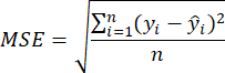
where y_i is the stress value before reversing standardization for the i-th sample point, is the predicted stress value before reversing standardization for the i-th sample, and n is the total number of samples.

The ANN's prediction of stress was very close to the FE simulation results, with an MSE of 0.0024. Predictions on four selected test cases are shown in Figure 5; the heat input for those four test cases are 333 J/mm, 538 J/mm, 692 J/mm, and 1222 J/mm, respectively. Among all these four cases, the ANN predictions show good agreement with the FE simulation results in general. However, in scenarios when the welding speed is 2.25 mm/s with a travel length of 50 mm and a net energy input rate of 2750 W or when the welding speed is 3.75 mm/s with a travel length of 40 mm and a net energy input rate of 1250 W, relatively big discrepancies are observed at the bottom of the BD line (near 17 mm depth). These discrepancies may be attributed to the increased complexity of the rules governing this region, resulting in a more intricate manifold within these specific parameter space regions. A possible solution would be to increase the density of the training dataset in this area.

Figure 1: Workflow. The proposed workflow has four steps (indicated in blue blocks): baseline FE model building, scripting, data generation, and surrogate model development. Orange blocks represent the input of each step, and green blocks represent the output of each step. Please click here to view a larger version of this figure.

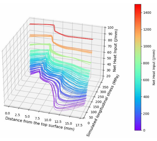
Figure 2: Generated dataset. A total of 205 sets of longitudinal stress data are illustrated, each corresponding to a unique combination of travel length, net energy input rate, and welding speed. Within each set, 20 data points are plotted for different nodes along the BD line. To differentiate between sets, each one is represented by a different color, which corresponds to its net heat input rate. This value can be calculated by dividing the net energy input rate by welding speed. This figure has been modified from²⁵. Please click here to view a larger version of this figure.

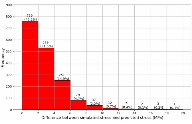
Figure 3: Frequency of the discrepancy between FE simulation results and ANN predictions. The differences between the FE simulation results and ANN predictions in the test dataset are categorized into 10 levels. The in-plot annotations indicate the frequency and percentage of occurrences for each level of difference in the test cases. Please click here to view a larger version of this figure.

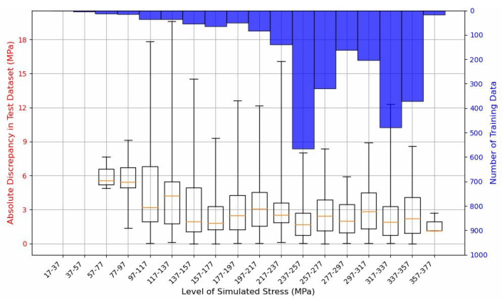
Figure 4: Distribution of average absolute residuals and training dataset across different stress levels. The box plot describes the distribution of absolute discrepancies between the simulated stress and the predicted stress for different levels of simulated stress. The orange line inside each box represents the median, indicating the midpoint of the absolute discrepancies. The height of each box corresponds to the interquartile range, which spans the middle 50% of the data (from the 25th to the 75th percentile), reflecting the variability of the discrepancies. The whiskers extend from the box to show the minimum and maximum values of discrepancy. The blue histogram shows the number of training data points corresponding to each stress level in the training dataset. Please click here to view a larger version of this figure.

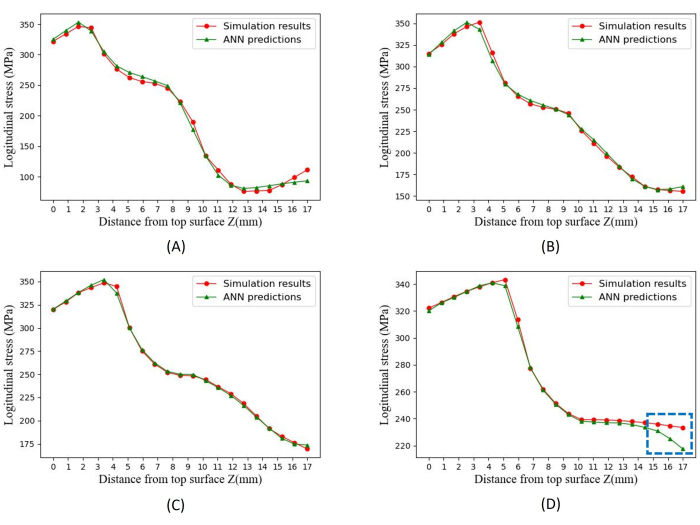
Figure 5: Comparison between simulation results and ANN predicted results. Four test cases are shown in this figure, with (A) welding speed is 3.75 mm/s, the travel length is 40 mm, and the net energy input rate is 1250 W; (B) welding speed is 3.25 mm/s, the travel length is 60 mm, and the net energy input rate is 1750 W; (C) welding speed is 3.25 mm/s, the travel length is 50 mm, and the net energy input rate is 2250 W; and (D) welding speed is 2.25 mm/s, the travel length is 50 mm, and the net energy input rate is 2750 W. The most notable discrepancy across all test cases is highlighted with a blue box, showing a difference of 19.4 MPa at a depth of 17 mm from the top surface in the test case (D). Please click here to view a larger version of this figure.

Table 1: Geometry information for weld specimen, refinement mesh region, and bead. The length, width, and depth of the rectangular weld specimen and refinement mesh region are listed in the table. The dimensions of the weld bead are illustrated with a sketch. In the modeling process, the width should be halved since only half of the model has been created. Please click here to download this Table.

Table 2: Material properties of AISI 316LN¹⁴. Density and Poisson's Ratio are treated as temperature-independent, and the other physical properties are treated as temperature-dependent. Please click here to download this Table.

Table 3: Plastic mechanical properties of AISI 316LN²⁴. Mechanical properties of AISI 316LN stainless steel as a function of temperature; yield stress at zero plastic strain; kinematic hardening parameters (C1, Gamma 1, C2, Gamma 2); isotropic hardening parameter (Q-inf); and hardening parameter (b). Please click here to download this Table.

Supplementary Coding File 1: Create_input_files.py Please click here to download this File.

Supplementary Coding File 2: Run_thermal Please click here to download this File.

Supplementary Coding File 3: DFLUX.for Please click here to download this File.

Supplementary Coding File 4:Run_Mechanical Please click here to download this File.

Supplementary Coding File 5: extract_data.py Please click here to download this File.

Supplementary Coding File 6: ANN_development.py Please click here to download this File.

Discussion

This study presents a workflow for automating data generation from finite element simulations and training machine learning-based surrogate models, such as artificial neural networks, to predict critical outcomes in welding processes. Firstly, the protocol involves building a standard weld finite element simulation to establish a consistent framework for reliable results. The simulation outcomes are analyzed and validated against experimental data to ensure accuracy. Secondly, scripts that can perform preprocessing and postprocessing of the simulation are developed based on recorded scripts using the macro function. Thirdly, large datasets are generated by using generated scripts. Lastly, a surrogate model is developed and tested, demonstrating its exceptional performance. This methodology contributes to the efficiency of the dataset generation process, eliminating the need for repetitive manual configurations. Recognizing the pivotal role of dataset generation in the development of data-driven surrogate models, the outlined workflow serves to expedite the surrogate model development process. Consequently, the presented methodology stands as a valuable resource for facilitating the development of data-driven surrogate models in the context of welding simulations.

In the protocol, several critical steps significantly influence the performance of the final surrogate model. In step 1.2.9, it is essential to ensure that the weld model incorporates sufficiently fine mesh elements to achieve stable convergence and accurate simulation results. In step 1.5.3, calibrating the standard finite element model enhances the appropriateness of the heat source model parameters selection and improves the simulation's accuracy. In steps 4.4 and 4.5, proper hyperparameter tuning is crucial for identifying the optimal model configuration, thereby enhancing the performance of the surrogate model.

The performance of the developed ANN surrogate model was evaluated, and it was found that it performed well overall. The accuracy of the surrogate model developed in this work is greater than previous attempts, which were based on very limited data^19,23. In the case study, the surrogate model developed is specifically designed for predicting longitudinal stress in a single weld bead-on-plate configuration, incorporating three key welding parameters: welding speed, travel length, and net energy input rate. It is important to note that both the inputs and outputs of the model are highly adaptable. For instance, additional welding parameters or material properties can be incorporated into the inputs, and the outputs can be expanded to encompass all residual stress components or displacement, offering a versatile framework for a broader range of applications.

As for the algorithm used for building the surrogate model, it is also modifiable based on the tasks. ANNs have some limitations for extrapolation. In contrast to ANNs, other machine learning algorithms, such as support vector machines (SVMs), are not limited by the structure of the training data and have a better ability of extrapolation. Previous studies^18,19,20 have attempted to use SVMs to predict residual stress with some success. However, it is important to note that it can be more challenging to tune SVM hyperparameters, and SVMs may not always perform well in interpolation tasks compared to ANNs. Another limitation of ANNs is that direct use of ANNs cannot generate a belief interval, which is of engineers' concern. Therefore, other algorithms, like Gaussian Process Regression²⁶ and Bayesian Neural Networks²⁷, can be considered. Furthermore, although the ANN model performs well in predicting residual stresses, it lacks interpretability. This lack of interpretability can be a drawback in engineering applications where understanding the model's decision-making process is crucial. The interpretability of the model can be improved by integrating more explanatory models, such as decision trees.

In conclusion, the proposed workflow in this study enables the rapid and easy generation of datasets, which can significantly accelerate the development of general or specific welding simulation surrogate models.

Materials

List of materials used in this article

Name	Company	Catalog Number	Comments
Abaqus	Dassault Systems	2020
Intel Fortran Compiler	Intel Corporation	17.0.7
Keras	Open Source	2.6.0
Python	Open Source	3.8.18

References

- Francis, J. A., Bhadeshia, H., Withers, P. J. Welding residual stresses in ferritic power plant steels. Mater Sci Technol. 23 (9), 1009-1020 (2007).
- Withers, P. J. Residual stress and its role in failure. Rep Prog Phys. 70 (12), 2211(2007).
- Hornbach, D. J., Preve´y, P. S. The effect of prior cold work on tensile residual stress development in nuclear weldments. J. Press Vessel Technol. 124 (3), 359-365 (2002).
- Zondi, M. C. Factors that affect welding-induced residual stress and distortions in pressure vessel steels and their mitigation techniques: a review. J Press Vessel Technol. 136 (4), 040801(2014).
- Ohms, C., Wimpory, R. C., Katsareas, D. E., Youtsos, A. G. NET TG1: Residual stress assessment by neutron diffraction and finite element modeling on a single bead weld on a steel plate. Int J Press Vessels Piping. 86 (1), 63-72 (2009).
- Bouchard, P. J. The NeT bead-on-plate benchmark for weld residual stress simulation. Int J Press Vessel Piping. 86 (1), 31-42 (2009).
- Hofmann, M., Wimpory, R. C. NET TG1: Residual stress analysis on a single bead weld on a steel plate using neutron diffraction at the new engineering instrument 'STRESS-SPEC'. Int J Press Vessels Piping. 86 (1), 122-125 (2009).
- Smith, M. C., Smith, A., Ohms, C., Wimpory, R. A review of the NeT TG4 international weld residual stress benchmark. ASME Press Vessels Piping Conf 2015. 6B, (2015).
- Akrivos, V., Smith, M. C. Material characterization on the nickel-based alloy 600/82 NeT-TG6 benchmark weldments. Proc ASME Press Vessels Piping Conf 2019. Uddin, M., Brongers, M., Messner, M. 6B, (2019).
- Wimpory, R. C., Ohms, C., Hofmann, M., Schneider, R., Youtsos, A. G. Statistical analysis of residual stress determinations using neutron diffraction. Int J Press Vessels Piping. 86 (1), 48-62 (2009).
- Ficquet, X., Smith, D. J., Truman, C. E., Kingston, E. J., Dennis, R. J. Measurement and prediction of residual stress in a bead-on-plate weld benchmark specimen. Int J Press Vessels Piping. 86 (1), 20-30 (2009).
- Gilles, P., El-Ahmar, W., Jullien, J. F. Robustness analyses of numerical simulation of fusion welding NeT-TG1 application:"Single weld-bead-on-plate.". Int J Press Vessels Piping. 86 (1), 3-12 (2009).
- Shan, X., Davies, C. M., Wangsdan, T., O'dowd, N. P., Nikbin, K. M. Thermo-mechanical modelling of a single-bead-on-plate weld using the finite element method. Int J Press Vessels Piping. 86 (1), 110-121 (2009).
- Bate, S. K., Charles, R., Warren, A. Finite element analysis of a single bead-on-plate specimen using SYSWELD. Int J Press Vessels Piping. 86 (1), 73-78 (2009).
- Coules, H. E., Smith, D. J., Venkata, K. A., Truman, C. E. A method for reconstruction of residual stress fields from measurements made in an incompatible region. Int J Solids Str. 51 (10), 1980-1990 (2014).
- Smith, M. C., Smith, A. C., Wimpory, R., Ohms, C. A review of the NeT Task Group 1 residual stress measurement and analysis round robin on a single weld bead-on-plate specimen. Int J Press Vessels Piping. 120, 93-140 (2014).
- Na, M. G., Kim, J. W., Lim, D. H. Prediction of residual stress for dissimilar metals welding at nuclear power plants using fuzzy neural network models. Nucl Eng Technol. 39 (4), 337-348 (2007).
- Na, M. G., Kim, J. W., Lim, D. H., Kang, Y. J. Residual stress prediction of dissimilar metals welding at NPPs using support vector regression. Nucl Eng Design. 238 (7), 1503-1510 (2008).
- Edwin Raja Dhas, J., Kumanan, S. Evolutionary fuzzy SVR modeling of weld residual stress. Appl Soft Comput J. 42, 423-430 (2016).
- Koo, Y. D., Yoo, K. H., Na, M. G. Estimation of residual stress in welding of dissimilar metals at nuclear power plants using cascaded support vector regression. Nucl Eng Technol. 49 (4), 817-824 (2017).
- Kitano, H., Nakamura, T. Predicting residual weld stress distribution with an adaptive neuro-fuzzy inference system. Int J Automat Technol. 12 (3), 290-296 (2018).
- Mathew, J., Griffin, J., Alamaniotis, M., Kanarachos, S., Fitzpatrick, M. E. Prediction of welding residual stresses using machine learning: Comparison between neural networks and neuro-fuzzy systems. Appl Soft Comput J. 70, 131-146 (2018).
- Liu, F., et al. Prediction of welding residual stress and deformation in electro-gas welding using artificial neural network. Mater Today Comm. 29 (May), 102786(2021).
- Muransky, O., Hamelin, C. J., Smith, M. C., Bendeich, P. J., Edwards, L. The effect of plasticity theory on predicted residual stress fields in numerical weld analyses. Computat Mater Sci. 54, 125-134 (2012).
- Miao, Z., Margetts, L., Vasileiou, A. N., Yin, H. Surrogate model development using simulation data to predict weld residual stress: A case study based on the NeT-TG1 benchmark. Int J Press Vessels Piping. 206, 105014(2023).
- Seeger, M. Gaussian processes for machine learning. Int J Neural Sys. 14 (02), 69-106 (2004).
- Chen, S. J., Zhang, Z. K. Temperature prediction of friction stir welding based on Bayesian neural network. Appl Mech Mater. 48, 1208-1212 (2011).
Reprints and Permissions