Serial Two-Photon Tomography of the Whole Marmoset Brain for Neuroanatomical Analyses

Summary

Serial two-photon tomography (STPT) imaging is a technique to image a mass of tissue in its three-dimensional shape by combining two-photon imaging with automatic stage control and microtome slicing. Here we describe a protocol for implementing it for marmoset brains to better understand their structural features.

Abstract

Serial Two-photon tomography (STPT) is a technique to image a mass of tissue in its three-dimensional shape by combining two-photon imaging with automatic stage control and microtome slicing. We successfully implemented this technique for tracing the axonal projections in the marmoset brain. Here, the detailed experimental procedures that resulted in reliable volumetric imaging of the whole marmoset brain are described. A key process for successful imaging was the removal of meninges surrounding the brain, which interferes with slicing. A big advantage of this methodology is that the sliced sections can be used for additional staining. In the original set-up, the sliced sections are scrambled in the water bath. These sections can be correctly aligned in their original order according to the blood vessel patterns in the cortex. An example of effective histology is the visualization of myelin structure by simple light reflection, which can be combined with Nissl staining to define anatomical borders. These sections can also be used for immunological detection of non-fluorescent anterograde and retrograde tracers, which can be registered to the STPT data for layering of multiple data.

Introduction

In neuroanatomical studies, researchers are faced with the need to observe micrometer-order structures (e.g., axons and boutons) in the context of the whole brain. This difficult task has been typically approached by visually inspecting the serial sections and looking for the region of interest for detailed imaging, analyses, and photo recording. With technological advancement, however, it is becoming possible to image the entire brain at high resolution for whole-brain analysis. In a ground-breaking study by Oh et al.¹, hundreds of mouse brains received tracer injections for connectomic analysis, which were processed by serial two-photon tomography (STPT) imaging technique². This study's characteristic was that they selected anterograde tracers to quantify "connectivity". While anterograde tracers provide very detailed spatial information on axonal distribution, neuroanatomists have relied on laborious manual segmentation for its analysis. By automating various analytical procedures, including this segmentation step, they succeeded in the "mass production" of ready-to-use high-resolution tracer data for multi-purpose uses. The effectiveness of their approach is obvious, given a variety of studies that used their tracer data^3,4,5 and their standard brain⁶.

Historically, the neural connectivity of non-human primate brains has attracted the attention of many neuroanatomists since the development of the degeneration method in the 1950s, to anterograde/retrograde substance transportation methods in the 1970s to the present viral strategy^7,8. As such, vast pieces of literature exist that investigate primate neural connections. In particular, many researchers have investigated the complex corticocortical connectivity of the macaque brain, and their results have been curated for tabulation (e.g., CoCoMac⁹). Although useful, these classic studies had several limitations. First, because each study focuses only on limited brain regions, the obtained information inevitably becomes fragmental. Second, each study uses different methods and conditions. Thus, the quantitative evaluation across studies becomes complicated. Third, the connectivity is usually shown either as a camera lucida of representative sections or as a semi-quantitative table/graph for author-defined brain regions. In other words, only very limited information from a complex brain structure is extracted for presentation in the published literature. With the development of magnetic resonance imaging (MRI) techniques, whole-brain studies at low resolution became prominent. However, there is a large gap between the levels of detail between what we know about neural connections in mice and those in primates.

With such background in mind, we set out to perform comprehensive anterograde tracing of the common marmoset brains^10,11. Although much smaller and smoother than the macaque brain, the marmoset counterpart exhibits clear signs of primates, such as the presence of area MT and the granular prefrontal areas, neither of which is clearly defined in rodents^12,13. Here, the small size was a big advantage because even the marmoset brain weighs ten times greater than the mouse brain. Fortunately, we could image the whole marmoset brain with minimal updates of the original version of TissueCyte1000 (henceforth referred to as a whole tissue imaging system) operating software, the commercially available microscope for STPT imaging². This update was to allow extra movement of the stage before slicing. The current version is now sufficient for processing the marmoset brain. This article shares a protocol to handle the marmoset brain for STPT imaging. The post-imaging protocol that further enhances the utility of this method is also provided.

Protocol

​All experimental procedures were carried out following the National Institute of Health Guide for the Care and Use of Laboratory Animals (NIH Publications No. 80-23) revised in 1996 and the Japanese Physiological Society's "Guiding Principles for the Care and Use of Animals in the Field of Physiological Science," and were approved by the Experimental Animal Committee of RIKEN (W2020-2-009(2)).

1. Tracer injection

1. Perform injections of fluorescent and non-fluorescent tracers to the marmoset brain according to previously reported procedures¹⁴.
   1. Regarding the combination with the STPT method, ensure that the fluorescence of the tracers is strong enough to be detected without enhancement. Adopt a double-vector TET-Off system¹⁰ for enhanced expression.
      NOTE: Non-fluorescent tracers can also be injected and detected after STPT is done using the produced slices. Examples of non-fluorescent tracers include Biotinylated Dextran Amine (BDA), cre-expressing AAV in AAV2 retro for retrograde detection of the input cell nuclei¹⁰, as well as GFP-based smFP-tag AAVs (see below).
2. Perfusion fix and obtain the marmoset brain after 4 weeks.
   1. To anesthetize the marmoset, administer Medetomidine (0.04 mg/kg), midazolam (0.4 mg/kg), and butorphanol (0.4 mg/kg), called MMB, intramuscularly, followed by intraperitoneal injection of Thiopental Sodium (100 mg/kg).
   2. After confirming that the pain reflex is lost, cut open the chest cavity to expose the heart and cut the right atrium to allow the blood and fixative to exit.
   3. Then cut the left ventricle to insert the perfusion needle for first flushing the blood with the prefix solution (250 mM sucrose, 5 mM MgCl₂ in 0.02 M phosphate buffer [PB, pH 7.4]) for a few minutes (~50-100 mL), followed by fixation with 4% paraformaldehyde/0.1 M phosphate buffer (PB; 2-3 times the weight of the animal over ~20 min).
   4. Good perfusion is critical for a good result. When inserting the perfusion needle, advance it along the septum toward the aorta to secure a good flow of the fixative. The tip of the needle becomes visible when it reaches the aorta. Retract until the tip is barely visible so it does not bypass the carotid artery.
3. Keep the brain in 4% paraformaldehyde/0.1 M PB for 48 h at 4 °C and transfer to 50 mM PB. If not used immediately, store the brain in 0.75% Glycine/0.1 M PB to prevent autofluorescence due to overfixation.

2. Sample preparation (Figure 1)

1. Incubate the fixed brain with collagenase (1 mg/mL in 3 mM CaCl₂ in 10 mL of tris buffered saline [TBS])at 37 °C for 1 h.
   NOTE: Prewarm the brain at 37 °C for 5 min before incubation.
2. Carefully rub the brain surface with a cotton swab to peel off the pia matter and other meninges (Figure 1A, Supplementary video). Use fine forceps to peel the detached meninges.
   NOTE: It is important to remove the meninges surrounding the midbrain, including the superior colliculus or those at the top of the thalamus. It is difficult to expose these structures that are hidden deep inside. However, remove meninges as much as possible. Otherwise, they often remain uncut, float up, and interfere with imaging and slicing (Figure 2A).
3. Take extra caution when the brain is subjected to ex vivo MRI before embedding, during which the brain is immersed in fluorine solution¹⁵. The leftover fluorine, if embedded together, could form tiny air bubbles under the objective while imaging. To avoid this, keep the brain in PB for 1 week before embedding.
   NOTE: This waiting step is usually not necessary but is critical when combined with ex vivo MRI.
4. Prepare the NaBH4 buffer by dissolving 0.2 g of NaBH4 in 100 mL of 50 mM borate buffer (pH 9.2) warmed to 40°C. Leave the cap loose to let the CO₂ gas out. Keep the solution overnight with the cap loosened. Wrap the bottle in aluminum foil to protect it from light until use.
5. Make oxidized agarose by stirring 2.25 g of agarose and 0.21 g of NaIO₄ in 100 mL of PB for 2-3 h. Filter the solution with vacuum suctioning and wash it with three changes of the PB. Resuspend the agarose in 50 mL of PB.
6. Completely melt the agarose in a microwave oven and cool to 60-65 °C.
7. Place the brain into a custom-made chamber and embed the brain in agarose. Take care to introduce the agarose into the cavity below the corpus callosum (Figure 1B).
   NOTE: Prewarm the brain first at room temperature and then at 65 °C for 5 min to allow the agarose to settle on the brain surface without solidifying.
8. Disassemble the chamber and immerse the agarose block in the NaBH4 buffer overnight at 4 °C.
9. Change the buffer to PB several times over 1-2 weeks at 4 °C.
   NOTE: The tissue autofluorescence becomes very weak if the buffer exchange is incomplete.
10. Make a slide glass stage by attaching four Neodymium magnets with epoxy instant mix.
11. Mount the agarose block onto the stage with a strong adhesive (e.g., super glue) (Figure 1C).

3. Tissue processing

1. Operate the whole tissue imaging system according to the manufacturer's instructions. A detailed protocol is also published¹⁶. The current procedure is mainly used for TissueCyte1000 but can be applied to other models, such as TissueCyte 1600FC.
2. The operation is slightly different between the models, but follow the points below that are commonly important.
   1. The entire marmoset brain can be processed coronally from the anterior to the posterior ends without any changes in the hardware. Ensure that the stage moving limits are not exceeded when placing the brain.
   2. Fine-tune the angle of the blades to ensure that the surface depths at both ends of the blade are within 10 µm. Because of dense myelination, even a 10 µm difference in depth could lead to different laser penetrations through adult marmoset white matter. For the same reason, set the imaging plane at about 25-35 µm from the surface.
   3. Use a ceramic blade (recommended) to cut the entire brain at 50 µm intervals (~over 650 slices).
   4. The meninges remain uncut and interfere with slicing if not properly removed (Figure 2). Some meninges (e.g., those surrounding the hippocampus or pulvinar) are difficult to remove. Manually extract these meninges by fine forceps when noticed.

4. Auxiliary histological techniques

1. Section retrieval
   1. Recover the tissue slices to perform various histological staining. Accurately align these sections in order of slicing. Trace the blood vessels across cortical layers for alignment (Figure 3).
2. Cut off excess agarose from each section for better handling.
   NOTE: This process needs not to be excessive. The agarose serves to hold tissue segments in place without interfering with the histological processing.
3. Backlit imaging
   1. Mount the sections onto a slide glass and dry.
   2. Rehydrate the section with PBS and place the coverslip for imaging.
   3. Observe a myelination pattern with no staining when the section is imaged by a fluorescence microscope (Figure 4) in a brightfield mode. Adjust the exposure time so that the light reflection can be visible.
      NOTE: Any microscope can be used if it can use dark field illumination.
   4. Remove the coverslip and proceed to Nissl staining or any other staining. Any standard staining procedure is sufficient.
   5. Use this method to directly compare different staining patterns with the myelination patterns (Figure 4).
4. BDA imaging
   1. See Table 1 for a detailed procedure.
   2. First, treat the sections with Dent's Solution (20% DMSO, 80% Methanol). Methanol included in Dent's solution dramatically enhances the BDA signals in the axons.
   3. Use the tyramide signal amplification (TSA) method to enhance the BDA signal to be fluorescently detected¹⁷.
      NOTE: TSA-biotin solution can be purchased from the vendor, but the In-House reagent is much cheaper and more effective.
   4. To register to the STPT image, take a backlit image after mounting the section to a slide glass with the mounting media.
5. Spaghetti monster fluorescent protein (smFP) staining
   NOTE: The 'spaghetti monster' fluorescent proteins (smFPs) are a family of non-fluorescent GFP variants with multiple epitope tags¹⁸. They provide excellent fluorescent signals upon immunodetection and are suitable as companion tracers to fluorescent tracers. See Table 2 for the AAV constructs available from Addgene.
   1. Follow the detailed procedure provided in Table 1.

5. Post-imaging data processing

1. Data integrity test
   NOTE: STPT generates a vast number of image files. When the brain of an adult marmoset is coronally sectioned at 50 µm intervals, more than 650 sections are typically required to cover the entire brain. Each section's data consists of a series of tiling images captured in three channels. These image files are stored in a single folder along with a metadata file that records the position of each tile. To minimize the total amount of data and processing time, imaging is conducted in blocks of runs, during which the number of X and Y steps for tiling gradually changes. Typically, 20-30 blocks of runs, each comprising the imaging of 30-50 sections, constitute the complete dataset for a single brain. To utilize this data, several image processing steps are required, including stitching of the tiled images, segmentation of fluorescent signals, and registration of the volumetric data to a standard template, among others.
   1. Perform the image processing steps individually using various software tools or through dedicated pipelines tailored to the researchers' specific needs. Details of the image processing are beyond the scope of this paper and can be found in other publications^11,19.
   2. Regardless of the procedure used, ensure that the data is organized consistently.
      NOTE: Since the entire imaging process involves many blocks of runs and spans several days, it is not uncommon for a run to be canceled midway and restarted anew. In such cases, the data structure can become disrupted, hindering the proper execution of the image processing pipeline.
   3. To minimize the risk of disruption of the data structure, run a Python script to check the integrity of the data structure (kn_pipeline_check_mosaic.py) available at GitHub (github.com/watkarbey/STPT_depo).
2. Registration of the stained image to the STPT image
   NOTE: Non-linear transformation of the stained image to the STPT image can be performed using the bUnwarpJ plugin of ImageJ.
   1. Adjust the size of the images of the target (STPT) and the source (stained) images so that they are approximately equal.
   2. Binarize each image to visualize the shapes of the sections.
   3. Run bUnwarpJ. Remember to check the Save Transformations option.
   4. Start bUnwarpJ again. Select the original image before binarization as the source image. Then click on Load Elastic Transformation and choose the saved transformation.

Results

In the typical set-up used here, the whole brain of an adult marmoset can be imaged (Figure 5) at the resolution of ~1.3 x 1.3 µm/pixel with a 50 µm section interval in about 1 week. This amounts to ~650 coronal images in three channels after image stitching. With a 16x objective lens (Nikon 16xW CFI75 LWD; NA = 0.80), the field of view of a single shot is about 1 x 1 mm. The image for the entire coronal surface is obtained by stitching these shots (Figure 5A). The alignment in the Z direction is excellent and a good 3D image is obtained by simply stacking the coronal image data (Figure 5B,E). For standardization, the STPT template for the marmoset brain¹¹ can be used for 3D-3D registration (Figure 5F). This data transformation is one of the key aspects of the whole brain neuroanatomy, in which a region of interest is assigned an absolute space coordinate independent of anatomical annotation. Once the sample brain is registered to the standard space, one can easily take out the subregions of interest for further analysis (Figure 5F,G). In particular, the cortical regions can be transformed into a flat map using a predetermined parameter (Figure 5H).

The sections generated during the imaging can be used for various histological purposes. As shown in Figure 4A,B, the backlit imaging with no staining provides a very similar pattern to the authentic myelin staining. This can be an excellent alternative to myelin staining. Furthermore, if the backlit image is obtained before Nissl staining, the same section can be used to obtain the patterns of both myelin and Nissl staining, thus providing useful information to identify areas and layers (Figure 5C-E). These sections can also be used for immunological staining. In Figure 5J, the section around the injection center was counterstained with NeuN antibody to estimate the transduction efficiency of the AAV virus. It is also a good strategy to inject non-fluorescent tracers in addition to fluorescent tracers and detect them histologically after section retrieval. In our previous study, we combined anterograde green tracers with retrograde "cre" vector, which was later detected by anti-cre antibody¹⁰. In an example of Figure 6A-E, BDA was injected into the contralateral side of the green tracer (clover) and fluorescently detected it. Note that the red BDA signals can be registered to the TissueCyte image to be localized in the whole brain coordinate. In another example of Figure 6F-I, smFP-myc was injected into the parietal area (Figure 6G), while the green tracer was injected into the frontal area. This way, multiple tracers can be injected into the same animal without interfering with the imaging. A big advantage of using the STPT sections for additional staining is that the relationship between the fluorescent and non-fluorescent tracers can be determined for the same brain. As such, we were able to determine the reciprocity of corticocortical projections at high-precision¹⁰. Another advantage is that the 3D coordinates of the stained sections can be mapped back to the STPT data and then to the standard template. Thus, it may not be necessary to use all the retrieved sections for staining. For better interpretation, sections can be selected for staining to add further context to the STPT data.

Figure 1: Sample preparation for STPT. (A) Meninge removal using cotton swabs. The meninges surrounding the brainstem can be removed by fine-tipped forceps. The meninges surrounding the marmoset brain are removed manually by rubbing with cotton swabs. The photo shows the meninges pealed from within the lateral sulcus. (B) The acryl box used for agarose embedding. The pins are movable and used to adjust the angle of the brain to be close to the stereotaxically fixed position²⁰. (C) A magnetic slide made of 76 mm x 52 mm slide glass and four Neodymium magnets attached by epoxy adhesive. The agarose block is attached to the magnetic stage with super glue. Please click here to view a larger version of this figure.

Figure 2: The effect of meninges on imaging. (A) Meninges that remain uncut float up, as shown by the white arrow. In this example, extensive protrusion of the meninges is seen because they were not removed before agarose embedding. Usually, meninges remain uncut only for several difficult regions. (B) An example of bad slicing due to the presence of meninges between the corpus callosum and the upper part of the thalamus. In this case, bad slicing led to the alternation of a deep slice (329) and a relatively normal slice (330). #78-329 stands for sample no. 78 section no. 329 in the Brain/MINDS data portal (C) Another example of bad imaging. In a worse case, the pulvinar nucleus shown by the red arrow may entirely come off. Scale bars: 0.5 mm (upper panel), 0.5 µm (lower panel). (D) Another example of bad imaging. The meninges deep within the calcarine sulcus is difficult to remove. The shadows seen in sections 469 and 470 are caused by the floating meninges that came under the objective. Scale bars: 0.5 mm (upper panel), 0.5 µm (lower panel). Please click here to view a larger version of this figure.

Figure 3: Alignment of tissue sections in order. (A) Up to 50 marmoset coronal sections can be correctly aligned in order in a plastic container (31 cm x 22.5 cm). To visualize the detailed structures, the container is placed on black paper and lighted from the side. These sections are first roughly aligned in order and then subject to precise alignment. (B) The precise alignment uses the blood vessel as the marker. The cerebral cortex contains many blood vessels that run vertically across cortical layers. They are identified as elongated holes that systematically change their positions within the cortical layers (white arrows). Using this method, even sections with 50 µm intervals can be accurately aligned. These blood vessel holes can be identified in the SPTP section images for confirmation. Scale bar: 5 mm (upper panel), 1 mm (lower panel). Please click here to view a larger version of this figure.

Figure 4: Backlit image as a substitute for the myelin staining. (A,B) The identical section was used for backlit imaging and myelin staining. First, the section was mounted onto the slide glass, dried, rehydrated with PBS, coverslipped, and imaged using a light microscope (Table of Materials). After removing the coverslip, the same section was used for myelin staining²¹ and imaged using a fluorescence microscope. The backlit image was registrated to the myelin image using the bUnwarpJ plugin of ImageJ. The green boxes show the magnified views of each image. Note that these images show almost identical patterns, except that the myelin staining visualizes fibrous structures better. (C-E) The identical section was used for backlit imaging and Nissl staining. The low-threshold mask for the backlit image was first registered with the low-threshold mask for the Nissl image using the bUnwarpJ plugin, and the original image was transformed using the same parameter. Note that the blood vessels (white arrowheads) are matched well between the two images. Because these two images are for the same section, the matching is almost perfect, and one can directly compare the myelin and Nissl patterns for the identification of cortical layers. Scale bars: 5 mm (panels A-E). Please click here to view a larger version of this figure.

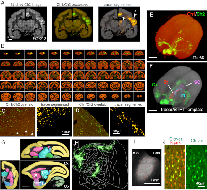
Figure 5: Typical result of STPT imaging. (A) A simple tiling of Ch2 (green) images of an example section (section 310 of sample #21). Without background correction, the borders for each tile are visible. In the middle column, the tiles were stitched with background correction for Ch1 (red) and Ch2 (green), respectively. To reduce the signals of lipofuscin (see panel C), Ch1 signals were subtracted from Ch2 and shown green. To reduce the lipofuscin signals of Ch1, the "Remove Outilers.." command was used before stitching by ImageJ. In the right column, the tracer signals were segmented by image processing pipeline¹¹. The arrowheads (c, d) show the locations where the magnified views are shown in panels C and D. Scale bar: 2 mm. (B) Overview of serial sections for sample #21. STPT generated 635 high-resolution coronal images for this sample. (C) A high magnification view shown by arrowhead c in panel A. This is a simple overlay of Ch1 (red) and Ch2 (green) with no further processing. The triangles show lipofuscin fluorescence signals, which show a widespread spectrum. The tracer segmentation algorithm accurately distinguishes the tracer signals from the lipofuscin background despite a very similar shape (right panel). Scale bar: 100 µm. (D) Another example of a high magnification view. Note that fine axon fibers in layer 1 can be well visible. Scale bar: 100 µm. (E) The 3D reconstruction of original STPT images. The 635 low-resolution coronal images as shown in panel B were used as the tiff-stack for 3D visualization using fluorender²². Scale bar: 5 mm. (F) The 3D reconstruction of the segmented tracer signals registered to the STPT template (grey). The tracer signals in different brain regions were shown by different colors. These regions were cut out by using the annotation shown in panel G. Scale bar: 5 mm. (G) STPT template overlaid with annotation of different brain regions. Scale bar: 5 mm. (H) The cortical tracer signal shown in panel F was shown in the form of a flatmap. (I) Identification of the injection site by the Ch3 fluorescence, which is less sensitive to the tracer fluorescence and remains unsaturated. Scale bar: 1 mm. (J) Staining the section around the injection center with NeuN antibody showed that approximately 30 % of the neurons show strong expression of Clover green fluorescence. Scale bar: 40 µm. Abbreviations: Cx; cortex, St; striatum, Th; thalamus, SC; superior colliculus. Amy; amygdala, Hip; hippocampus, Cb; cerebellum. Please click here to view a larger version of this figure.

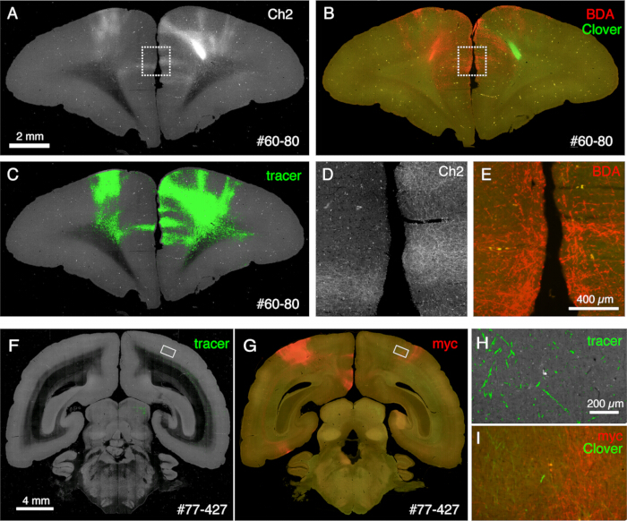
Figure 6: Post-STPT histology showing multiple non-fluorescent tracers. (A-C) Comparison of STPT image with BDA-stained image. In this sample, BDA is injected into the contralateral side of Clover injection. Panels A and C show the Ch2 image and tracer segmentation of the STPT data. Panel B shows the post-STPT staining for BDA. Clover fluorescence is diminished due to the methanol treatment of the section. Scale bar: 2 mm. (D,E) The dotted boxes in panels A and B are magnified. Scale bar: 100 µm. (F,G) Comparison of STPT image with anti-myc tag antibody staining. In this sample, Clover injection is to the PFC, whereas the AAV-smFP-myc is injected into the contralateral parietal cortex. The white rectangles are magnified in panels H and I. Scale bar: 4 mm. (H) Tracer segmentation is shown in green. Scale bar: 200 µm. (I) The myc staining is shown in red. The Clover fluorescence is shown in green. Scale bar: 200 µm. The green signals in panels H and I are present in a similar position but not identical because STPT retrieves only ~10 µm optical section. Please click here to view a larger version of this figure.

BDA fluorescent staining protocol
Remove agarose
TBS wash	10 min (2x)
1% H2O2 in Dent's solution	10 min
TBS wash	Brief
0.5% TNB  blocking	1 h
StAvHRP (1:4000) in TNB	2 overnight
TNT wash	10 min (3x)
TSA Biotin (1:4000) in 0.1 M borate (pH8.5) + 0.003% H2O2	2 h
TNT wash	10 min (3x)
Cy3-streptavidin  (1:1000) in TNT	3 h
TNT wash	10 min (2x)
TBS wash	Keep the section until mounting
Mount section onto slideglass using an antifade mounting medium
anti-myc fluorescent staining protocol
Remove agarose
TBS wash	10 min (2x)
blocking in IB	1 h
Anti-Myc (1:4000) in IB	2 over night
TNT wash	10 min (3x)
Anti-mouse Cy3 (1:1000) in TNT	3 h
TNT wash	10 min (2x)
TBS wash	Keep the section until mounting
Mount section onto slideglass using an antifade mounting medium
Buffers/solutions	Composition
0.5% TNB	0.5% TSA Blocking Reagent in TS7.5
Dent's Solution	20% DMSO, 80% Methanol
Immersion buffer (IB)	10% FBS, 2% BSA 0.5% TritonX100 in TBS
TBS (Tris-buffered saline)	25 mM Tris, 137 mM NaCl, 2.7 mM KCl (pH 7.4)
TNT	0.05 % Tween20  in TS7.5
TS7.5	0.1 M TRIS-HCl, pH 7.5, 0.15 M NaCl

Table 1: BDA fluorescent staining and anti-myc fluorescent staining protocol

Plasmid for AAV tracer	Addgene No.	Recommended antibody	Suggested dilution	Expected result
pAAV-EF1_Cre	201198	Millipore clone 2D8	1:1000	good for cells
pAAVCam1.3_smFP_Myc	201205	MBL M192 My3 (mouse)	1:4000	excellent
pAAVCam1.3_smFP_HA	201206	CST C29F4 (rabbit)	1:1000	good for cells
pAAVCam1.3_smFP_FLAG	201207	MBL PM020B (rabbit)	1:1000	OK
AAVTRE3_smFP_Myc	201208
AAVTRE3_smFP_HA	201209
AAVTRE3_smFP_FLAG	201210

Table 2: List of Addgene plasmids available for the production of non-fluorescent tracers. The cre construct targets the nucleus and is suitable for retrograde tracing enveloped by AAV2 retro. smFP_HA construct is good for cell body detection (and retrograde).

Supplementary Video: Microscope view of meninges removal. Please click here to download this Video.

Discussion

This article explained the practical solutions to handle marmoset brains for whole-brain processing as well as auxiliary histological techniques that enhance the utility of the STPT technique. The strength of "whole brain neuroanatomy" using STPT is that you can obtain the 3D coordinates of any region of interest, whether it is anatomically annotated or not. By high-precision 3D-to-3D registration, it is possible to transform these coordinates into a standard template for the overlay of multiple datasets. This way, the standard template serves as the medium of data integration. This was an essential aspect of our prefrontal cortex (PFC) mapping project¹⁰, where data obtained from many individuals were analyzed. Furthermore, the information mapped to the standard template can be compared with various data that have already been mapped, whether it is Nissl, myelin patterns, tracer data, MRI (including diffusion MRI) data, or anatomical annotations¹¹. Importantly, it can also be compared with future data that will be gained by yet-to-emerge technology. There currently exist multiple templates for the marmoset brain, which are based on Nissl staining²³, MRI^{23,24,25,26,27,28}, and STPT¹¹. But they can be transformed to each other's coordinates based on image contrasts and precalculated parameters¹¹. Data integration at the whole brain scale across studies contributes to a better understanding the brain as a system. The prerequisite for this strategy to work is reliable data acquisition across the brain. Below, critical steps and potential problems associated with the current protocol are discussed.

One of the most vulnerable processes of STPT imaging is tissue slicing. As mentioned above, the meninges often remain uncut and can interfere with the slicing. In particular, the pulvinar nucleus and the superior colliculus are the two most affected brain regions: depending on the thoroughness of meninge removal and embedding in agarose, they can be stripped off from the tissue block during slicing. These deep regions are difficult to approach from the outside and can easily break during meninge removal. A careful but thorough meninge removal is critical for successful imaging. Another concern is the flip back of sliced sections onto the tissue block, which sometimes occurs when the sections remain attached even after slicing. It can be minimized by shaping the block so that the blade cuts obliquely at the very end.

By imaging deep into the tissue block, STPT avoids the bumpiness of its surface. Whereas the fluorescent signals can pass through the cortical region rather easily, they are highly diminished in the myelinated regions. Therefore, the imaging depth needs to be carefully determined to balance between the consistent imaging across the entire block surface and the brightness of the signals in the myelin-rich region, such as the white matter. In the setup used here, we usually aim at 25-35 µm from the surface. It also needs to be cautioned that the cut surface may become unevenly shrunk after long hours of storage. To minimize the imaging area, we split the imaging session into 20-30 runs with different stage settings for 5-6 days. We either make the interval between runs less than 2 h or confirm the surface depth and adjust the stage height before each run.

In this protocol, the BDA signal was amplified by the TSA method. This method is highly effective and can detect anterogradely transported BDA signals even at relatively low resolution (e.g., Figure 6B). TSA biotin is commercially available from Akoya Biosciences, but the homemade solution shows much better enhancement. On the other hand, the dilution of the antibody and solution requires careful adjustment to obtain the optimal result. Pretreatment of the section with a methanol solution is critical. Without pretreatment, the BDA signals are barely detected in the myelinated axons.

When an anterograde tracer is used, it is often difficult to identify the exact site of injection because of the saturation of the fluorescence signals. In the whole tissue imaging system setup used in this study, we use the blue channel to identify the infected cells (Figure 5I). Even when the red and green channels are saturated, each individual infected neuron is usually detectable in the blue channel. This is also true with the Allen Mouse Brain Connectivity Atlas¹. Examination of the cells of origin is important because the infection sometimes involves only particular layers. We encountered such partial infections rather frequently for the Mouse Brain Connectivity Atlas, perhaps because of the utilization of the iontophoresis method²⁹. The lateral spread of the viral tracers could be more or less variable depending on the injections. This variability can potentially affect the result of tracing and needs careful normalization.

The successful registration of the obtained 3D image to the standard template is a key process of the whole brain neuroanatomy. Registration of the STPT image to the STPT template can be pretty accurate, and we observed only deviances of a few voxels (50 µm isocubic) for the borders with a high image contrast¹⁰. Still, there is a limit to what registration can do. Because of the meninge removal process, the STPT samples generally have gaps between the hemispheres and between the cortex and midbrain/hindbrain, whereas brain tissues are tightly packed in the in vivo MRI images. Such differences are difficult to adjust by registration. The Marmoset cortex is mostly devoid of sulci, but the intraparietal sulcus is very deep in some Individuals. Such a sulci will be lost (top-to-top fusion occurs) upon registration. Although registration is a powerful technique, it is necessary to go back to the raw data for confirmation of the obtained result.

The generation of massive image data is both a strength and a limitation of this technique. While it enhances the completeness of the dataset, it necessitates careful management of the acquired data and the development of an automated image processing pipeline for efficient data interpretation. In the future, the application of generative artificial intelligence (AI) in constructing image processing pipelines may significantly simplify this process. Systematic whole-brain imaging has also been performed using slide scanner-based methods^21,30. Compared to such methods, STPT does not require additional computation for 3D reconstruction. Combined with optical sectioning, we have demonstrated that STPT has the potential to reconstruct even axon segments across sections³¹. With the further combination of tissue clearance techniques, Economo et al. developed a method to image the entirety of sparsely labeled neurons^32,33. The latest versions of TissueCyte now offer options for an additional laser to enhance the excitation of red fluorescent proteins or a section capture unit for the automatic recovery of sections. With these advancements, the whole-brain approach will become more efficient, providing a foundation for a comprehensive understanding of the primate brain, including that of humans.

Materials

List of materials used in this article

Name	Company	Catalog Number	Comments
Agarose type I	Sigma	A6013
All-in-one fluorescence microscope	Keyence	BZ-X series	This study used BZ-X710
anti-mouse Cy3	Jackson Immuno Research Laboratories, Inc.	115-165-003
anti-myc antibody	MBL	M192	mouse monoclonal
Butorphanol	Meiji Animal Health	Vetorphale
Ceramic blade	TissueVision	N/A
Collagenase type I	Wako Chemical	#031-17601	Aliquot into 100 µL x 10 of 100 mg/mL in PBS
Cotton swab (HUBY-340)	HUBY	BB-013SP	micro cotton swabs
Custom-made chamber	N/A	N/A	The chamber consist of four side plates and one bottom plates, all made of 1 cm thick acrylic plates, which can be securely fastened together using screw bolts. An additional acrylic plate is placed inside the chamber, with three metal poles  inserted through it to hold the marmoset brain in an inverted position.
Cy3-Streptavidin	Jackson Immuno Research Laboratories, Inc.	016-160-084
Dumont #5 forceps, Inox	N/A	N/A
Epoxy instant mix	Locktite	N/A
FIJI	NIH	https://imagej.net/software/fiji/downloads
kn_pipeline_check_mosaic.py	N/A	N/A	github.com/watkarbey/STPT_depo; This is a checking script for TissueCyte data.
Medetomidine	Zenoaq	Domitor
Midazolam	Sandoz	N/A
NaBH4	Sigma	#452882
NaIO4	Sigma	S1878
Perfusion needle	Natsume Seisakusho Co., Ltd	KN-348, 20G-50
Slideglass (76 mm x 52 mm)	Matsunami	S9111
StAvHRP	Jackson Immuno Research Laboratories, Inc.	016-030-084	HRP-streptavidin (titration needs to be carefully determined)
TissueCyte1000	TissueVision	https://www.tissuevision.com/tissuecyte
TSA blocking reagent	Kiko Tech	FP1012	Refer to TSA-biotin kit (Akoya Biosciences)
TSA-biotin	House-made	N/A	See Okamoto et al (ref. 16)
VECTASHIELD HardSet Mounting Medium	Vector laboratories Inc	N/A	Antifade mounting medium

References

- Oh, S. W., Harris, J. A., Ng, L., Winslow, B., Cain, N., et al. A mesoscale connectome of the mouse brain. Nature. 508 (7495), 207-214 (2014).
- Ragan, T., et al. Serial two-photon tomography for automated ex vivo mouse brain imaging. Nat Methods. 9 (3), 255-258 (2012).
- Liang, Z., Arefin, T. M., Lee, C. H., Zhang, J. Using mesoscopic tract-tracing data to guide the estimation of fiber orientation distributions in the mouse brain from diffusion MRI. Neuroimage. 270, 119999(2023).
- Watakabe, A., Hirokawa, J. Cortical networks of the mouse brain elaborate within the gray matter. Brain Struct Funct. 223 (8), 3633-3652 (2018).
- Ypma, R. J. F., Bullmore, E. T. Statistical analysis of tract-tracing experiments demonstrates a dense, complex cortical network in the mouse. PLoS Comput Biol. 12 (9), e1005104(2016).
- Wang, Q., et al. The Allen mouse brain common coordinate framework: A 3D reference atlas. Cell. 181 (4), 936-953.e20 (2020).
- Köbbert, C., Apps, R., Bechmann, I., Lanciego, J. L., Mey, J., Thanos, S. Current concepts in neuroanatomical tracing. Prog Neurobiol. 62 (4), 327-351 (2000).
- Lanciego, J. L., Wouterlood, F. G. Neuroanatomical tract-tracing techniques that did go viral. Brain Struct Funct. 225 (4), 1193-1224 (2020).
- Bakker, R., Wachtler, T., Diesmann, M. CoCoMac 2.0 and the future of tract-tracing databases. Front Neuroinform. 6, (2012).
- Watakabe, A., et al. Local and long-distance organization of prefrontal cortex circuits in the marmoset brain. Neuron. 111 (14), 2258-2273.e10 (2023).
- Skibbe, H., et al. The Brain/MINDS marmoset connectivity resource: An open-access platform for cellular-level tracing and tractography in the primate brain. PLoS Biol. 21 (6), e3002158(2023).
- Mitchell, J. F., Leopold, D. A. The marmoset monkey as a model for visual neuroscience. Neurosci Res. 93, 20-46 (2015).
- Okano, H. Current status of and perspectives on the application of marmosets in neurobiology. Annu Rev Neurosci. 44, 27-48 (2021).
- Watakabe, A., et al. Comparative analyses of adeno-associated viral vector serotypes 1, 2, 5, 8 and 9 in marmoset, mouse and macaque cerebral cortex. Neurosci Res. 93, 144-157 (2015).
- Hata, J., et al. Multi-modal brain magnetic resonance imaging database covering marmosets with a wide age range. Sci Data. 10, 221(2023).
- Liwang, J. K., Bennett, H. C., Pi, H. -J., Kim, Y. Protocol for using serial two-photon tomography to map cell types and cerebrovasculature at single-cell resolution in the whole adult mouse brain. STAR Protoc. 4 (1), 102048(2023).
- Okamoto, S., et al. Exclusive labeling of direct and indirect pathway neurons in the mouse neostriatum by an adeno-associated virus vector with Cre/lox system. STAR Protoc. 2 (1), 100230(2021).
- Viswanathan, S., et al. High-performance probes for light and electron microscopy. Nat Methods. 12 (6), 568-576 (2015).
- Kuan, L., et al. Neuroinformatics of the Allen mouse brain connectivity atlas. Methods. 73, 4-17 (2015).
- Paxinos, G., Watson, C., Petrides, M., Rosa, M., Tokuno, H. The Marmoset Brain in Stereotaxic Coordinates. , Academic Press. London, Waltham, MA. (2012).
- Abe, H., et al. 3D reconstruction of brain section images for creating axonal projection maps in marmosets. J Neurosci Methods. 286, 102-113 (2017).
- Wan, Y., et al. FluoRender: Joint freehand segmentation and visualization for many-channel fluorescence data analysis. BMC Bioinformatics. 18 (1), 280(2017).
- Majka, P., et al. Towards a comprehensive atlas of cortical connections in a primate brain: Mapping tracer injection studies of the common marmoset into a reference digital template. J Comp Neurol. 524 (11), 2161-2181 (2016).
- Liu, C., Yen, C. C. -C., Szczupak, D., Tian, X., Glen, D., Silva, A. C. Marmoset brain mapping V3: Population multi-modal standard volumetric and surface-based templates. Neuroimage. 226, 117620(2021).
- Liu, C., et al. A digital 3D atlas of the marmoset brain based on multi-modal MRI. Neuroimage. 169, 106-116 (2018).
- Liu, C., et al. A resource for the detailed 3D mapping of white matter pathways in the marmoset brain. Nat Neurosci. 23 (2), 271-280 (2020).
- Woodward, A., et al. The Brain/MINDS 3D digital marmoset brain atlas. Sci Data. 5, 180009(2018).
- Saleem, K. S., Avram, A. V., Glen, D., Schram, V., Basser, P. J. The subcortical atlas of the marmoset ("SAM") monkey based on high-resolution MRI and histology. Cereb Cortex. 34 (4), bhae120(2024).
- Lin, M. K., et al. A high-throughput neurohistological pipeline for brain-wide mesoscale connectivity mapping of the common marmoset. eLife. 8, e40042(2019).
- Skibbe, H., et al. PAT-probabilistic axon tracking for densely labeled neurons in large 3-D micrographs. IEEE Trans Med Imaging. 38 (1), 69-78 (2019).
- Economo, M. N., et al. A platform for brain-wide imaging and reconstruction of individual neurons. eLife. 5, e10566(2016).
- Winnubst, J., et al. Reconstruction of 1,000 projection neurons reveals new cell types and organization of long-range connectivity in the mouse brain. Cell. 179 (1), 268-281.e13 (2019).
Reprints and Permissions