Ultrasound Localization Microscopy for Super-Resolution Mapping of the Rodent Brain Microvasculature

Summary

Ultrasound Localization Microscopy (ULM) is a recently developed technique that allows for an unprecedented level of resolution in imaging the microvasculature in vivo. In this work, we describe in detail how to obtain super-resolved images of the brain microvasculature in rodents using a standardized functional ultrasound imaging platform designed for preclinical research.

Abstract

Ultrasound Localization Microscopy (ULM) is a super-resolution imaging technique that enables in vivo visualization of the brain's microvascular architecture surpassing the diffraction limit of conventional ultrasound. By detecting and tracking intravenously injected microbubbles as they circulate through cerebral vessels, ULM produces high-resolution maps of vascular density, flow velocity, and backscattered signal amplitude at spatial scales down to 5-10 µm. This protocol presents a complete workflow for performing ULM imaging in rodents, including animal preparation, probe positioning, image acquisition, microbubble injection, and data processing, using a dedicated functional ultrasound platform. Two preparation methods are described, adapted for mice (transcranial) and rats (with cranial windows), followed by detailed instructions for probe alignment and anatomical targeting using an integrated brain atlas. During acquisition, ultrafast ultrasound sequences are synchronized with bolus injections of microbubbles to capture dynamic flow data. Subsequent reconstruction steps involve clutter filtering, image interpolation, microbubble detection, subpixel localization, and trajectory tracking. Outputs include density maps reflecting vessel occupancy, velocity maps revealing flow patterns and directionality, and amplitude maps offering additional contrast for structural interpretation. Representative results illustrate successful acquisition across full coronal planes and highlight common pitfalls such as poor injection quality, motion artifacts, and skull-induced aberration. The protocol is compatible with both cross-sectional and longitudinal studies and is particularly suited for investigating cerebrovascular alterations in models of aging, stroke, aneurysm, and neurodegenerative diseases. By combining depth penetration, high spatiotemporal resolution, and label-free vascular imaging, ULM offers a powerful tool for noninvasive brain microcirculation analysis in preclinical models.

Introduction

Though the brain accounts for only 2% of the body's mass, it consumes around 20% of its oxygen and glucose to sustain neuronal activity¹. This high metabolic demand is met by an intricate vascular network, from large arteries and veins to microvessels like arterioles, venules, and capillaries, regulated through neurovascular coupling². The disruption of this finely tuned process has been implicated in a broad spectrum of neurological disorders. Neurovascular uncoupling, for instance, is an early pathological feature in diseases such as Alzheimer's, Parkinson's, Huntington's, and Amyotrophic Lateral Sclerosis (ALS), often preceding the classical hallmarks of neurodegeneration such as amyloid-beta and tau pathology^3,4,5,6. Imaging the brain's complex nature in vivo has therefore been of primary concern to address the growing need to understand physiological processes. Technological advancements have provided unique capabilities to probe brain function and activity, both directly and indirectly, with increasing precision, resolution, and accessibility.

Doppler ultrasound has emerged as a powerful tool for the functional measurement of brain activity using blood flow⁷. In particular, power Doppler imaging, designed to detect the motion of red blood cells (RBCs), transmits repeated ultrasonic pulses to blood vessels and records the amplitude of ultrasonic echoes backscattered by moving RBCs⁸. The advent of ultrafast ultrasound imaging, specifically functional ultrasound (fUS), marked a pivotal point in overcoming previous limitations. Indeed, conventional ultrasound scans tissue line by line-a sequential approach that confines its application to the major cerebral arteries, as the slow blood flows typical of the brain's microvasculature cannot be detected⁹. The more recent fUS technique uses multiple plane-wave transmissions to acquire thousands of frames per second, dramatically improving both the temporal resolution and signal-to-noise ratio (SNR). Crucially, fUS enables the detection of hemodynamic changes in very small vessels with velocities as low as 1 mm/s, supporting real-time functional imaging of brain activity down to the level of arterioles⁸.

While ultrafast Doppler methods have significantly improved microvascular imaging, they are still constrained by the diffraction-limited resolution of ultrasound¹⁰. In tandem with fUS, ultrasound localization microscopy (ULM) breaks through this impediment, enabling the visualization of microvascular structures at the capillary level by leveraging contrast agents and high-precision localization algorithms¹¹. This provides unprecedented insights into vascular morphology and function. More specifically, in ULM, contrast agents made of stabilized gas-filled microbubbles, approximately 1-3 µm in diameter, are injected into the bloodstream. They act as strong acoustic scatterers that can be detected as individual point sources. Given that microbubbles are significantly smaller than the ultrasound wavelength, they can be spatially and temporally isolated, appearing as the system's point-spread function (PSF). Inspired by optical super-resolution techniques such as STORM and PALM, sub-pixel localization of these microbubbles is achieved using deconvolution methods that map their positions with high precision^10,12,13,14. This allows vascular structures to be resolved at a spatial resolution of 5-10 µm, well beyond the diffraction-imposed limit of conventional ultrafast ultrasound power Doppler imaging.

ULM is a powerful and effective tool for vascular mapping down to the capillary scale and overcomes the limitations of many optical methods that are restricted to superficial layers. Its ability to perform microvascular imaging in living animals, allowing for longitudinal and pharmacological studies, is another key advantage of ULM over other techniques that require brain fixation and staining. The extracted information extends beyond static vascular maps, providing quantitative estimates of blood flow down to the capillary level, thereby opening promising avenues for both preclinical and clinical applications. To facilitate reproducibility, we describe a full workflow for ULM-based brain imaging in rodents, implemented using a standardized functional ultrasound imaging platform designed for preclinical research.

Protocol

All procedures described in this study were conducted in compliance with the European Community Council Directive of 22 September 2010 (010/63/UE) and approved by the local ethics committee (Comité d'éthique en matière d'expérimentation animale number 59, 'Paris Centre et Sud', project #2020-16). Experiments were carried out on adult male C57BL/6 Rj mice (2 months old, 20-30 g) and Sprague-Dawley Rj:Han rats (200-300 g) sourced commercially. Animals were housed in groups of four per cage under a 12-h light/dark cycle, with a constant temperature of 22 °C, and with food and water provided ad libitum. Prior to the start of the experiments, all animals underwent a minimum one-week acclimatization period to the housing conditions. The reagents and the equipment used are listed in the Table of Materials.

1. Animal preparation

1. Anesthesia and animal preparation in mice
   1. Place the mouse in the isoflurane induction chamber, administering 2% isoflurane with air (0.075 L/min) and oxygen (0.175 L/min, or medical air).
   2. Confirm adequate anesthesia depth by checking for the absence of reflexes in response to a toe or tail pinch using firm but non-damaging pressure. If a reflex is present, increase the isoflurane concentration slightly. Reassess before proceeding.
   3. Transfer the animal to the stereotaxic frame, which is placed over a heating pad set at 37 °C to maintain body temperature, and ensure continuous Isoflurane delivery via a mask at the same concentration and flow rate.
   4. Apply eye ointment to prevent eye ulceration and cataract formation.
   5. Shave the mouse's head using a trimmer. Apply a depilatory cream, let it sit 1 to 1.5 min maximum, then rinse thoroughly with warm water and dry with gauze. Repeat as needed until all hair is removed. Avoid leaving the depilatory cream for longer periods of time, as it may cause chemical damage to the skin.
   6. Apply centrifuged ultrasound gel (bubble-free, degassed) onto the head to ensure acoustic coupling.
2. Anesthesia and animal preparation in rats
   1. After weighing the rat, administer an intraperitoneal injection of a mixture of ketamine (75 mg/kg) and xylazine (10 mg/kg) using a 1 mL syringe. Shave the fur on top of the head and clean the skin with an iodine solution.
      NOTE: Ketamine is a highly regulated substance in many countries and may require special authorization for procurement and use. Alternative anesthetic regimens, including isoflurane, can be used to achieve surgical-level anesthesia.
   2. Position the animal on a stereotaxic apparatus that is placed over a heating pad set to 37 °C to maintain body temperature. Apply a generous amount of ophthalmic ointment to the eyes to prevent drying and cataract formation.
   3. Subcutaneously inject meloxicam (2 mg/kg) using a 1 mL syringe for intraoperative analgesia.
   4. Confirm adequate anesthesia depth by checking for the absence of reflexes in response to a toe pinch or tail pinch using firm but non-damaging pressure. If a reflex is present, administer an additional dose equal to one-fourth of the initial anesthetic dose. Wait approximately 5 min before reassessing anesthesia depth. Proceed only once a surgical plane of anesthesia is confirmed and reassess every 20-30 min.
   5. Make a longitudinal incision along the sagittal suture using a scalpel, ensuring the cut is deep enough to include the skin and connective tissues attached to the skull.
   6. Keep the surrounding tissues well hydrated throughout the surgery using physiological saline.
   7. Using a rotary drill, lightly trace the outline of the cranial window by marking the surface layer of the skull. For optimal access to the brain, the window should be around 14 mm in the lateral dimension and at least 2 mm in the anteroposterior dimension, depending on skull size.
   8. Continue milling along the outline until no bone resistance remains. During drilling, periodically apply a few drops of physiological saline to cool the bone and minimize thermal damage. A fine, round-edged spatula should be easily inserted into the gap without force.
   9. Using short, one-way reaming strokes, thin the last layer of bone until resistance is barely perceptible.
   10. Insert a thin, slightly curved spatula with rounded edges at the lateral edge of the cranial window.
   11. Slowly move the spatula toward the center, gently detaching the bone from the meninges. Once no resistance is felt, lift and fully remove the detached bone piece.
   12. Apply centrifuged ultrasound gel on top of the dura. A description of the experimental setup is depicted in Figure 1.

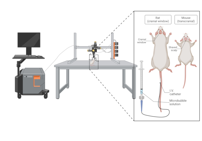
Figure 1: Schematic of the experimental setup for ULM brain imaging in rodents. The imaging system consists of an ultrasound acquisition unit connected to a high-frequency probe mounted on a motorized positioning stage. Both mice and rats are shown in stereotaxic frames: the mouse features a shaved scalp for transcranial imaging, while the rat undergoes imaging through a surgically prepared cranial window. A tail vein catheter is placed for contrast agent injection in both species. This setup allows for the stable acquisition of high-resolution functional ultrasound data during microbubble injection. Please click here to view a larger version of this figure.

3. Tail vein catheterization for mice or rats
   1. Use a 27 G × 1/2" winged infusion set connected to an 18 G × 1/2" needle with 8" tubing. Shorten the tubing, if possible, to minimize dead volume.
   2. Gently turn the animal's tail 90 degrees to expose the lateral tail veins (see Figure 2). Secure the tail in place using tape to ensure stability and prevent unnecessary movement during catheterization.
   3. Identify the tail vein by starting at the distal end (tip of the tail) and moving toward the base. To facilitate this step, the tail can be warmed with lukewarm water to promote vasodilation and enhance vein visibility.
   4. Using a finger, apply gentle pressure at the base of the tail and slide it toward the injection site (i.e., against the direction of blood flow). This maneuver temporarily impedes venous return, causing the caudal veins to distend and become more prominent, facilitating catheter insertion.
   5. Insert the 27 G × 1/2" needle of the winged infusion set parallel to the vein, ensuring the bevel is facing up.
   6. Observe the tubing for the presence of blood flashback, which confirms correct needle placement.
      NOTE: Begin catheterization at the distal tail end to avoid leakage from earlier punctures during subsequent injections. If tail vein catheterization proves challenging or unsuccessful, alternative central routes can be considered. These include the retro-orbital sinus/plexus, the jugular vein, or the saphenous vein.

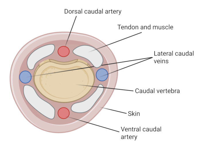
Figure 2: Cross-sectional anatomy of the rodent tail illustrating vascular landmarks for catheterization. A schematic drawing of a transverse section through the distal rodent tail, showing the relative positions of the major blood vessels. Two arteries are present near the midline: the dorsal caudal artery, located in the upper (dorsal) region, and the ventral caudal artery, positioned in the lower (ventral) part of the tail cross-section. These arteries are typically avoided during intravenous procedures. Flanking the arteries laterally are the caudal veins, which run symmetrically on either side and lie just beneath the skin, making them the preferred access sites for catheterization or microbubble injection. This anatomical overview assists in the precise localization of the veins, especially when enhanced by warming to promote vasodilation. Please click here to view a larger version of this figure.

4. Probe positioning using the IcoScan software
   1. On the acquisition platform, start the fUS acquisition software (e.g., IcoScan for Iconeus One) and create an experiment session. Adjust the ultrasound probe position.
      NOTE: Position the probe approximately 1 mm above the head of the rat or mouse. Ensure that the probe is in contact with the ultrasound gel before starting any imaging sequence.
   2. Start the Live View acquisition and adjust the probe position as needed using real-time cerebral blood volume (CBV) imaging. The brain should be centered on the image. Optimize imaging parameters, such as contrast and compression, to enhance visualization quality.
   3. Open the Angio3D menu in the acquisition software. Adjust the scanning parameters (First Slice, Last Slice, and Step Size), ensuring they cover the entire brain. Start the acquisition.
      NOTE: When setting up the scan parameters, ensure that the scan covers the posterior part of the brain, namely the entire posterior arteries.
   4. Keep the acquisition software open and start the IcoStudio software for data analysis and visualization. Load the Angio3D scan.
   5. Go to the Brain Registration panel and register the scan to the Allen Mouse Common Coordinate Framework using either the fully automatic or manual registration mode.
   6. Save the registration as a .bps file.
   7. Next, go to the Brain Navigation menu. In the Atlas Manager panel, use the Parent/Child tree navigator to browse the Allen Mouse Brain Atlas. Select the targeted anatomical regions, which will be superimposed onto the scan in the 3-view panel.
   8. Choose an imaging plane that overlaps the regions of interest. Manually set two markers in the coronal view to define the targeted imaging slice.
   9. Click on the Brain Positioning System (BPS) to extract the motor coordinates corresponding to the probe position for imaging the selected plane. Check the image preview, computed from the Angio3D scan, and click on Copy BPS Coordinates.
   10. Switch to the IcoScan software and open the Probe Positioning panel. Click on Enter BPS Coordinates and paste the values extracted in step 1.4.9. The probe will automatically move and align with the selected imaging plane.
   11. Perform a Live View acquisition to confirm that the current imaging plane matches the predicted plane from step 1.4.8.
       NOTE: By saving and reusing the same spatial markers, the imaging plane can be consistently redefined across sessions, enabling accurate probe repositioning for longitudinal studies.

2. ULM acquisition

1. Microbubbles preparation
   NOTE: A variety of commercially available ultrasound contrast agents can be used. However, the gas composition, bubble concentration, diameter, and stability may vary depending on the product used. Please follow the manufacturer's recommendations regarding preparation and storage.
   1. Using a sterile syringe, inject 5 mL of 0.9% sodium chloride solution into the vial through the septum.
      NOTE: For repeated bolus administrations or continuous infusion, a lower volume of 0.9% sodium chloride solution can be used to prepare a more concentrated microbubble suspension. Adjust the dilution factor accordingly based on the intended application.
   2. Agitate the vial vigorously for 20 s to fully resuspend the microbubbles and achieve uniform dispersion.
2. ULM recording
   1. Predefine the recording parameters, including the ultrasound sequence, frame rate, and total recording time.
      NOTE: Recommended parameters for recording are 5-10 min at 2.5 Hz.
   2. Draw the volume of microbubbles to be injected and start the acquisition. Once the acquisition has started, proceed with the microbubble injection. Injecting 200 µL for rats and 100 µL for mice, at the appropriate dilution, is recommended.
   3. Confirm the contrast enhancement on the Live View image. Immediately afterwards, flush the remaining microbubbles in the dead volume by injecting physiological fluid into the catheter. A typical example of a microbubble intensity profile is shown in Figure 3.
   4. Wait for the acquisition to complete and save the data.
   5. At the end of the acquisition, proceed as follows, depending on the protocol used:
      1. For mice (noninvasive protocol): Reverse the anesthesia by stopping isoflurane administration and monitor the animal during recovery in a warm environment until fully awake.
      2. For rats (invasive protocol with cranial window): Euthanize the animal by intraperitoneal injection of Euthasol (pentobarbital sodium, 140 mg/kg), in accordance with institutional and ethical guidelines.

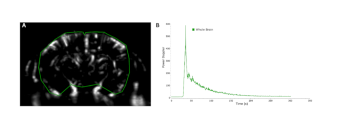
Figure 3: Microbubble signal intensity over time. (A) Illustration of the region of interest (ROI) used for signal extraction, encompassing the entire coronal brain slice. (B) Time course of microbubble signal intensity during a 5-min acquisition. The microbubble bolus was injected at 30 s, resulting in a characteristic rise in signal amplitude. Please click here to view a larger version of this figure.

3. Image reconstruction using the IcoLab software

1. Open IcoLab and navigate to ULM by clicking on the ULM tab on the leftmost part of the screen.
2. Click on Compute ULM Maps to initiate the processing workflow, as detailed in Figure 4.
3. Select the source folder containing the acquired data.
4. Choose the specific scan to be processed and adjust the processing time boundaries if needed.
5. Click on Next to proceed to the Reporting step. In the Reporting step, configure the output folder path where processed files will be saved. Set the visualization parameters for the images that will be included in the PowerPoint report.
6. Review the summary of selected options displayed on the final screen.
7. When ready, click on RUN to start the processing. Once the processing is complete, a .trk file will be generated, containing all the coordinates of localized microbubbles, along with rasterized TIFF files for density, velocity, and backscattered amplitude (BSA).
   NOTE: A 5 min acquisition may require several hours of processing. This step is best performed overnight or on a dedicated workstation.
   1. Generation of microbubble density maps: Localized positions of all detected microbubbles are accumulated over the selected acquisition time. Map these positions onto a fixed-resolution spatial grid.
      NOTE: Each pixel in the resulting density map reflects the count of microbubbles localized within that spatial bin. The final output is a grayscale image (TIFF) where pixel intensity corresponds to vessel occupancy, enabling high-resolution reconstruction of the vascular network.
   2. Generation of velocity maps: The software tracks individual microbubbles across consecutive frames to form trajectories. For each trajectory, the software computes a velocity vector by dividing the displacement by the elapsed time (yielding a velocity vector in mm/s).
      NOTE: Two types of velocity maps can be generated: absolute velocity maps, where each pixel stores the average speed magnitude of microbubbles passing through, and directional velocity maps, where velocity is decomposed along a chosen anatomical axis (i.e., x or z), and the corresponding signed component is stored. These maps are rasterized onto the same spatial grid and saved as individual TIFF images.
   3. Generation of BSA maps: For each localized microbubble, the raw ultrasound signal amplitude (backscattered intensity) is displayed. Project these amplitudes onto the spatial grid, accumulating the signal intensity in each pixel. The resulting BSA map highlights regions where microbubbles passed through the focal area of the beam, providing contrast that complements the density and velocity maps¹⁵.

Figure 4: Flowchart of the processing pipeline for ULM map reconstruction. The figure illustrates the sequential processing steps performed in the analysis software to generate ULM maps from raw ultrasound data. Starting from compounded frames (n = 200), Step 1 applies singular value decomposition (SVD) clutter filtering to isolate microbubble (MB) signals from the tissue background. In Step 2, the MB signals undergo Lanczos interpolation, resulting in a preprocessed image stack. Step 3 performs local maxima detection and correlates these with the system's point spread function (PSF) to identify candidate microbubble locations. In Step 4, subpixel localization (centroid detection) and particle tracking are used to extract microbubble trajectories, from which maps of velocity and backscattered amplitude are computed. Please click here to view a larger version of this figure.

4. Data visualization using the IcoStudio software

1. Load a .trk file in IcoStudio to begin data exploration.
2. Adjust visualization parameters such as contrast, compression, and colormap in the right-side panel to refine data representation.
3. Set the integration time by using the double slider at the bottom of the main view to define the start and end frames.
4. Open the Density tab to view microbubble occurrences and select between Absolute Density (count per pixel) and Directional Density (axially weighted).
5. Use the Velocity tab to display microbubble speed in mm/s through multiple modes: Absolute, Directional, Axial, and Lateral. Adjust contrast, compression, and velocity thresholds to enhance visualization.
6. Explore the BSA tab to visualize microbubble reflectivity, providing an alternative contrast mechanism that highlights microvascular structures and out-of-plane motion. Export high-resolution PNG screenshots or generate TIFF files for quantitative analysis with customizable pixel size and data type settings.

Results

The representative examples in Figure 5 show a typical example of ULM data of a rat brain acquired over 1 min of recording following 200 µL of microbubble bolus injection, with a 10 µm resolution.

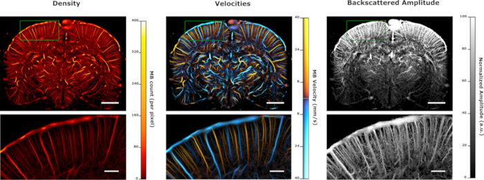
Figure 5: Representative ULM outputs acquired from a craniotomized rat following a single microbubble injection. Example maps of microbubble (MB) density (left), velocity (center), and backscattered amplitude (right) are shown for a full coronal brain slice, acquired over 1 min of recording following a 200 µL bolus injection of microbubbles. Scale bar: 2mm. Zoomed insets highlight the left cortical microvasculature (scale bar: 0.5 mm). The density map reflects the spatial distribution of MB occurrences, revealing the structure of the vascular network. The velocity map illustrates flow speed and directionality of individual MBs, enabling differentiation between vessel types. The amplitude map shows the backscattered ultrasound signal from MBs, providing an additional contrast mechanism that enhances visualization of vessel morphology and out-of-plane motion. Please click here to view a larger version of this figure.

The resulting maps illustrate three complementary views of the cerebral microvasculature: microbubble (MB) density (left), velocity (center), and backscattered amplitude (right). Each map corresponds to a full coronal slice of the brain, with zoomed insets highlighting the left cortical microvasculature (scale bars: 2 mm and 0.5 mm, respectively).

The density map shows the spatial distribution of MB occurrences across the field of view. Vessel morphology is resolved far below the diffraction limit, revealing both large vessels and fine capillary structures. This type of map enables clear visualization of vascular network topology, including bifurcations and branching patterns, even in deep cortical regions.

The velocity map displays the flow speed of individual MBs projected along the axial (z) direction. This projection produces signed velocity values, where negative velocities reflect upward flow into the cortex and positive values reflect downward flow. In the rodent cerebral cortex, the vascular architecture is highly stereotyped: penetrating arterioles descend from the pial surface into the cortical layers, while venules ascend from the cortex back to the surface to drain deoxygenated blood¹⁶. This consistent anatomical arrangement enables the use of directional velocity measurements to distinguish between vessel types, with positive axial velocities typically indicating arterial flow and negative velocities indicating venous drainage. Overall, the velocity values measured with ULM are consistent with previously reported ranges in the literature^10,17, spanning from 10-20 mm/s in penetrating arterioles to several centimeters per second in major intracranial arteries. These findings are in line with earlier observations that flowing microbubbles closely mimic the rheological behavior of red blood cells¹⁸, validating the use of ULM for quantifying physiological blood flow dynamics at the microscale.

The backscattered amplitude (BSA) map provides a spatial representation of the ultrasound signal intensity returned by each MB. As backscattered energy is maximized when MBs pass through the focal region, this map offers contrast based on elevational position. It helps refine segmentation by identifying out-of-plane motion or low-amplitude vessels, particularly at greater depths or near the focal edges. BSA maps are also valuable for detecting depth-related signal attenuation or identifying mismatches in focal alignment¹⁵.

To demonstrate the reproducibility of plane targeting with the Brain Positioning System, Figure 6A shows ULM vascular density maps acquired in the same mouse under anesthesia on day 0 (Week 1) and day 7 (Week 2), targeting the same coronal plane. The overlay of both maps shows a strong spatial correspondence of the vascular signal, confirming the precision of plane repositioning and the reliability of longitudinal experiments, as previously shown¹⁹.

Quantitative analysis can be applied to any of these outputs. For instance, users may segment vessels using intensity thresholds or clustering algorithms, and then extract regional statistics such as vessel density, average flow speed, and morphometric parameters including vessel radius, average length, number of branches, and other structural descriptors of the vascular network. Comparisons across cortical regions or experimental groups (e.g., drug-injected vs. control) can be performed directly on these maps or through derived parametric statistics on commonly identified vessels^20,21. As an example of such analysis, we performed regional quantifications of vascular parameters in the left somatosensory cortex (S1BF, Figure 6B) and left thalamus (Figure 6C). The density maps were first binarized, skeletonized, and vessel radii were estimated using a Euclidean distance transform. Flow velocities were directly obtained from the MB trajectories, and flow rate was derived from the vessel radius using Poiseuille's law as previously detailed²¹. The same methodology as described in that study was applied here. Whisker plots display the distributions of vessel radius, velocity, and flow rate for d0 and d7, demonstrating good reproducibility across sessions. Together, these multimodal ULM outputs enable comprehensive characterization of the brain's microvascular network, offering both anatomical and dynamic insights with unprecedented resolution.

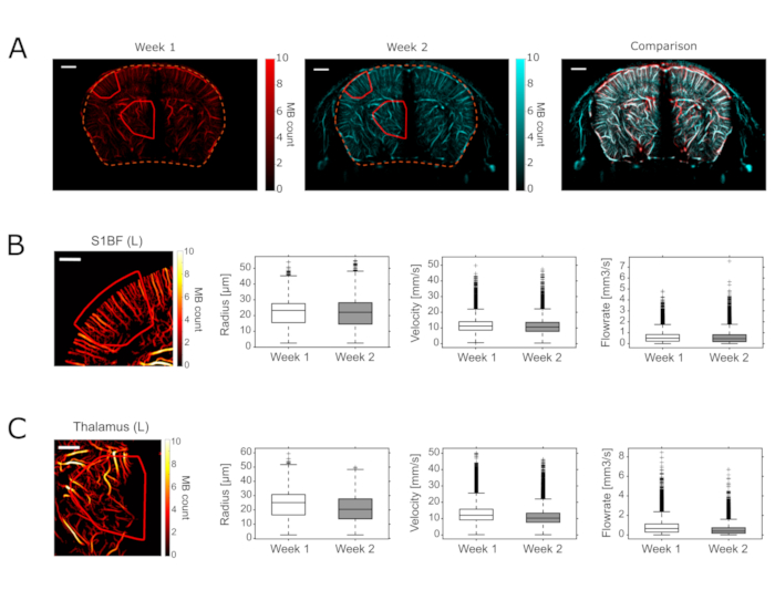
Figure 6: Longitudinal reproducibility of plane targeting and example of vascular quantifications using the Brain Positioning System. (A) ULM vascular density maps acquired from the same anesthetized mouse on day 0 (Week 1) and day 7 (Week 2), targeting the same coronal plane using the Brain Positioning System (scale bar = 1 cm). The overlay of both maps shows a strong spatial correspondence of the vascular signal, illustrating the reproducibility of plane positioning across sessions. (B,C) Representative quantification of vascular parameters extracted from two regions of interest: left somatosensory cortex (S1BF, B) and left thalamus (C). For each region, we display the vascular density map at d0 (scale bar = 0.5 cm), together with whisker plots showing the distribution of vessel radius (µm), flow velocity (mm/s), and flow rate (mm³/s) at d0 and d7 (median, 25th-75th percentile, whiskers = 1.5×IQR, outliers plotted individually). These results illustrate the ability of the pipeline to extract morphometric and hemodynamic metrics from the ULM data. Please click here to view a larger version of this figure.

Discussion

Ultrasound Localization Microscopy (ULM) represents a transformative advancement in ultrasound imaging, enabling super-resolution visualization of the microvasculature beyond the conventional diffraction limit. This discussion highlights the critical steps in the ULM protocol, addresses potential modifications and troubleshooting strategies, explores the limitations of the method, evaluates its significance compared to alternative imaging modalities, and considers its importance and potential applications in biomedical research.

Critical steps in the ULM protocol

Several steps are crucial to the successful implementation of ULM, and their influence is illustrated in Figure 7. One of the most important steps is the administration of microbubbles, as both the concentration and delivery quality directly affect imaging outcomes. An optimal concentration is necessary to balance spatial resolution and detectability. Inadequate delivery, such as poor catheter placement or extravasation, can result in very low vascular signal and incomplete reconstructions, as shown in Figure 7B, where only a sparse number of microbubbles reach the bloodstream. High-frame-rate imaging, typically in the kilohertz range, is essential for capturing the rapid movement of microbubbles and enabling reliable tracking across frames. Any instability during the acquisition, such as motion introduced by breathing, poor fixation, or insufficient anesthesia, can degrade the localization accuracy. An example of this is illustrated in Figure 7C, where excessive motion during the acquisition results in a blurred and unusable density map.

Microbubble localization and tracking depend on advanced image processing algorithms that detect individual bubbles, perform subpixel localization, and reconstruct trajectories with sub-diffraction precision. Even with proper acquisition and processing, anatomical factors such as skull-induced aberrations can still affect image quality. In transcranial imaging, particularly in older mice, skull thickening can introduce acoustic distortion. This leads to characteristic shadowing artifacts beneath the sagittal suture, where no microbubbles are detected, as depicted in Figure 7D. Such aberrations reduce signal-to-noise ratio and can obscure vascular structures unless corrected with adaptive filtering or by refining probe placement.

When all steps are performed successfully, high-quality ULM maps are achievable, as shown in Figure 7A, where a dense and well-resolved vascular network is reconstructed through a transcranial approach.

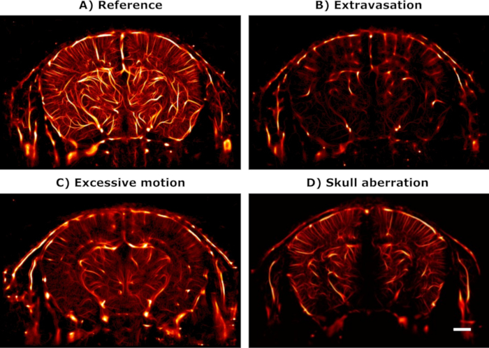
Figure 7: Reference and troubleshooting examples for ULM imaging quality in mice. Panel (A) shows a high-quality transcranial ULM microbubble (MB) density map acquired in a young adult mouse, illustrating successful vascular mapping across the full coronal plane. Panel (B) displays an example of a poor vascular signal due to microbubble extravasation or insufficient venous access, resulting in sparse MB detections. Panel (C) shows an acquisition affected by excessive animal motion, producing a blurry and non-interpretable density map. Panel (D) highlights skull-induced acoustic aberration commonly observed in older mice, visible as a shadow cone beneath the sagittal suture where no MBs are detected due to reduced signal-to-noise ratio. These examples serve as visual references for identifying and addressing common experimental artifacts in ULM imaging. Scale bar: 1mm. Please click here to view a larger version of this figure.

Limitations of the method

Despite its many advantages, ULM has inherent limitations that affect its applicability. Out-of-plane vessel bias is a significant issue in 2D imaging, as vessels extending outside the imaging plane are not adequately reconstructed, leading to incomplete vascular maps. This limitation can be mitigated by transitioning to volumetric (3D) imaging approaches²², although this increases computational complexity. Intravenous catheterization challenges also pose a hurdle, especially in small animal models, where achieving consistent microbubble delivery can be technically demanding. Microbubble stability is also a limiting factor, especially during extended imaging sessions. Due to their short circulation half-life, microbubbles may require repeated bolus injections or continuous infusion protocols to maintain adequate contrast throughout the acquisition period. Motion artifacts remain a significant concern, particularly for awake subjects, where even small involuntary movements can degrade super-resolution imaging. Finally, depth penetration in ULM is inherently limited by ultrasound attenuation. While this is generally not problematic for rodent imaging at high frequencies (e.g., 15 MHz), it becomes more challenging in larger animals such as swine or non-human primates. In these cases, lower-frequency probes may be required to achieve sufficient imaging depth, but this comes at the cost of reduced spatial resolution-underscoring a key trade-off between depth and detail that must be considered when translating ULM to larger preclinical models.

Significance of ULM compared to existing methods

Ultrasound Localization Microscopy (ULM) offers substantial advantages over conventional imaging modalities, particularly in the context of microvascular imaging. Among its most notable strengths is its ability to surpass the diffraction limit of traditional ultrasound, achieving sub-diffraction imaging at spatial scales comparable to optical techniques such as two-photon microscopy. Unlike these optical methods, however, ULM provides deeper tissue penetration, allowing access to brain regions that are otherwise difficult to visualize noninvasively.

ULM also offers functional imaging capabilities, enabling the quantitative assessment of blood flow velocity, perfusion dynamics, and vascular remodeling. These features make it highly suitable for investigating both physiological processes and pathological changes in neurovascular networks. Compared to MRI and PET, ULM is more cost-effective, does not require heavy infrastructure, and avoids the use of contrast agents with known toxicity risks, relying instead on gas-filled microbubbles with favorable safety profiles.

The combination of high spatial and temporal resolution makes ULM particularly valuable for a range of research applications. It is especially powerful in studies targeting microvascular structures and deep brain nuclei, where traditional modalities often fall short. Moreover, unlike histological approaches that require tissue fixation and staining, ULM enables real-time imaging in living animals, supporting longitudinal designs and dynamic interventions such as pharmacological challenges.

Beyond static vascular mapping, ULM also enables high-resolution functional imaging by capturing cerebral blood flow dynamics with exceptional spatial and temporal precision. Recent advances have demonstrated its feasibility for whole-brain functional neuroimaging in rodents, revealing stimulus-evoked and spontaneous activity-dependent changes in blood flow at the capillary level across distributed brain networks². This positions ULM as a powerful tool for functional studies, effectively bridging the gap between mesoscale hemodynamic imaging and neuronal activity mapping.

Usability, efficiency, and reproducibility considerations

The ULM workflow described in this protocol has been optimized for ease of implementation and reproducibility across different experimental setups. The use of commercially available components, including FDA- and EMA-approved microbubbles and standard rodent anesthesia procedures, ensures wide accessibility. In addition, the integration of the entire processing pipeline within the dedicated software (IcoLab) greatly enhances usability by automating complex steps such as microbubble localization, trajectory reconstruction, and map generation. This streamlined interface reduces the need for custom code and minimizes user intervention, supporting consistent results across users and experiments. While high-resolution ULM processing is computationally intensive, especially for long acquisitions or volumetric data, batch-processing tools and GPU acceleration significantly reduce analysis time. The protocol's modular design also supports reproducibility, allowing researchers to fine-tune acquisition and processing parameters while maintaining a robust analytical framework. The protocol also includes a dedicated section on probe positioning using IcoScan and IcoStudio, which enables users to reliably reposition the probe at the exact same imaging slice across sessions, with an accuracy of approximately 100 µm. This feature is particularly valuable for longitudinal studies, where precise spatial consistency is essential for tracking vascular changes over time. These features collectively lower the barrier to entry for new users and support the scalable deployment of ULM in both exploratory and longitudinal imaging studies.

Conclusion

This protocol presents a complete workflow for implementing Ultrasound Localization Microscopy (ULM) in rodent brain imaging, covering surgical preparation, microbubble administration, image acquisition, and high-resolution vascular mapping using a standardized acquisition and analysis platform optimized for preclinical research. ULM represents a major advance in biomedical imaging, offering super-resolution in vivo visualization of the microvasculature with unprecedented detail. Compared to existing imaging modalities, ULM provides a unique combination of high spatial resolution, functional flow quantification, and accessibility, making it especially well-suited for studies of vascular development, neurovascular coupling, and disease pathophysiology. As the technology continues to mature, ULM is poised to become a cornerstone in both preclinical research and, eventually, clinical neuroimaging applications.

Materials

List of materials used in this article

Name	Company	Catalog Number	Comments
Animal temperature controller (heating plate coupled with a rectal probe)	Physitemp	TCAT-2DF
Atipamezole	Orion Pharma, France	Antisedan	5 mg/mL injectable solution
C57BL/6 mice	Janvier Labs	SC-C57J-M	C57BL/6Rj male mice, 8 weeks old
Dental drill	Foredom, USA	K.1070 High Speed Rotary Micromotor Kit
Depilatory cream	Vichy	N/A
Eye ointment	TVM, UK	Ocry-gel
Hair trimmer	Phymep	ISIS GT 421 Aesculap
IcoLab processing software (v 1.2.0.0)	Iconeus, France	IcoLab
Iconeus One Xpand configuration	Iconeus, France	IconeusOne Xpand
IcoPrime 15MHz Probe	Iconeus, France	IcoPrime-15MHz Probe
IcoScan acquisition software (v1.9.0)	Iconeus, France	IcoScan
IcoStudio analysis software (v2.2.0)	Iconeus, France	IcoStudio
Iodine solution	Mylan, France	N/A
Isoflurane anesthesia station	Minerve, Esternay, France	N/A
Ketamine	Virbac, France	Ketamine1000	100 mg/mL injectable solution
Meloxicam	Boehringer Ingelheim	Metacam	0.5 mg/mL injectable solution
Needles	Terumo, France	AN*1838R1	18 G x ½” needle with 8” tubing
Saline water	Laboratoire Gilbert Physiodose, Pharmacy, France	N/A
Scalpel	DREXCO medical, France	80011
SonoVue microbubbles	Bracco Imaging	SonoVue 8ul/ml
Spatula	Phymed, France.	K.1070 High Speed Rotary Micromotor Kit
Sprague-Dawley Rj:Han rats	Janvier Labs	RN-SD-M	RjHan:SD - Sprague Dawley male rats, 200-300 g
Stereotaxic frame	David Kopf (Tujunga, USA)	900-WA	Using Mouse Adaptor  (Ref: 922) and Non-Rupture Ear Bars (ref: 922)
Syringe	DREXCO medical, France	2058
Ultrasound gel	DREXCO medical, France	Medi'Gel
Winged infusion set	Terumo, France	SV*27EL
Xylazine 2%	Bayer, France	Rompun	20 mg/mL injectable solution

References

- Jamadar, S. D., Behler, A., Deery, H., Breakspear, M. The metabolic costs of cognition. Trends Cogn Sci. 29 (6), 541-555 (2025).
- Renaudin, N., et al. Functional ultrasound localization microscopy reveals brain-wide neurovascular activity on a microscopic scale. Nat Methods. 19 (8), 1004-1012 (2022).
- Agarwal, N., Carare, R. O. Cerebral Vessels: An overview of anatomy, physiology, and role in the drainage of fluids and solutes. Front Neurol. 11, 611485(2021).
- Ahmad, A., Patel, V., Xiao, J., Khan, M. M. The role of neurovascular system in neurodegenerative diseases. Mol Neurobiol. 57 (11), 4373-4393 (2020).
- Sweeney, M. D., Kisler, K., Montagne, A., Toga, A. W., Zlokovic, B. V. The role of brain vasculature in neurodegenerative disorders. Nat Neurosci. 21 (10), 1318-1331 (2018).
- Kolinko, Y., Krakorova, K., Cendelin, J., Tonar, Z., Kralickova, M. Microcirculation of the brain: Morphological assessment in degenerative diseases and restoration processes. Rev Neurosci. 26 (1), 75-93 (2015).
- Deffieux, T., Demene, C., Pernot, M., Tanter, M. Functional ultrasound neuroimaging: A review of the preclinical and clinical state of the art. Curr Opin in Neurobiol. 50, 128-135 (2018).
- Mace, E., et al. Functional ultrasound imaging of the brain: Theory and basic principles. IEEE Trans Ultrason Ferroelectr Freq Control. 60 (3), 492-506 (2013).
- Tanter, M., Fink, M. Ultrafast imaging in biomedical ultrasound. IEEE Trans Ultrason Ferroelectr Freq Control. 61 (1), 102-119 (2014).
- Errico, C., et al. Ultrafast ultrasound localization microscopy for deep super-resolution vascular imaging. Nature. 527 (7579), 499-502 (2015).
- Réaux-Le-Goazigo, A., et al. Ultrasound localization microscopy and functional ultrasound imaging reveal atypical features of the trigeminal ganglion vasculature. Commun Biol. 5 (1), 330(2022).
- Siepmann, M., Schmitz, G., Bzyl, J., Palmowski, M., Kiessling, F. Imaging tumor vascularity by tracing single microbubbles. IEEE Int Ultrason Symp. , 1906-1908 (2011).
- Couture, O., Hingot, V., Heiles, B., Muleki-Seya, P., Tanter, M. Ultrasound localization microscopy and super-resolution: A state of the art. IEEE Trans Ultrason Ferroelectr Freq Control. 65 (8), 1304-1320 (2018).
- Dencks, S., Schmitz, G. Ultrasound localization microscopy. Z Med Phys. 33 (3), 292-308 (2023).
- Renaudin, N., Pezet, S., Ialy-Radio, N., Demene, C., Tanter, M. Backscattering amplitude in ultrasound localization microscopy. Sci Rep. 13 (1), 11477(2023).
- Blinder, P., et al. The cortical angiome: An interconnected vascular network with noncolumnar patterns of blood flow. Nat Neurosci. 16 (7), 889-897 (2013).
- van Raaij, M. E., et al. Quantification of blood flow and volume in arterioles and venules of the rat cerebral cortex using functional micro-ultrasound. Neuroimage. 63 (3), 1030-1037 (2012).
- Lindner, J., Song, J., Jayaweera, A. R., Sklenar, J., Kaul, S. Microvascular rheology of definity microbubbles after intra-arterial and intravenous administration. J Am Soc Echocardiogr. 15 (5), 396-403 (2002).
- Nouhoum, M., et al. A functional ultrasound brain GPS for automatic vascular-based neuronavigation. Sci Rep. 11, 15197(2021).
- Lowerison, M. R., et al. Super-resolution ultrasound reveals cerebrovascular impairment in a mouse model of Alzheimer's disease. J Endocrinol. 44 (9), 1-14 (2024).
- Nyúl-Tóth, A., et al. Novel intravital approaches to quantify deep vascular structure and perfusion in the aging mouse brain using ultrasound localization microscopy (ULM). J Cereb Blood Flow Metab. 0 (0), 1-19 (2024).
- Demeulenaere, O., et al. In vivo whole brain microvascular imaging in mice using transcranial 3D Ultrasound Localization Microscopy. EBioMedicine. 79 (1), 103995(2022).
Reprints and Permissions