High-plex Imaging using Spectral Confocal Microscopy to Minimize Non-specific Tissue Fluorescence

Summary

Spectral Iterative Bleaching Extends Multiplexity (IBEX) builds upon the base IBEX technique by adding heparin blocking to minimize nonspecific binding and leveraging spectral detection with computational unmixing to suppress autofluorescence. This approach accelerates image acquisition while reducing sources of background, enabling robust multi-round, high-parameter spatial proteomic analyses.

Abstract

Highly multiplexed imaging enables the study of functionally diverse cells and their niches within their native tissue environments. Iterative Bleaching Extends Multiplexity (IBEX) is a cyclic immunolabeling and fluorophore inactivation technique that allows for multiple markers to be visualized on the same tissue section. Captured images can be subsequently analyzed to acquire single-cell data to define cell clusters, their localizations, and neighboring cell types. Interpreting these data relies on the ability to distinguish true marker expressions from sources of background inherent to fluorescence microscopy. Spectral IBEX, an adaptation of the IBEX protocol, integrates spectral confocal detection with computational unmixing and incorporates heparin blocking to reduce charge-based off-target binding. This combination improves the signal-to-background ratio, suppresses tissue autofluorescence, and minimizes bleed-through while also reducing acquisition time compared to conventional multi-track confocal imaging. Application to human nasal polyp tissue, a model characterized by high eosinophil content and strong autofluorescence, demonstrated reliable imaging of 26 markers across structural, immune, and cell state compartments over six imaging rounds. The resulting workflow generates high-dimensional, spatially resolved proteomic information that captures complex tissue architecture and cellular niches. Together, this optimized approach provides a robust and broadly applicable strategy for multiplexed imaging, particularly suited to tissues where autofluorescence and non-specific staining limit conventional approaches.

Introduction

Tissues are comprised of a diverse set of cells with specialized functions that organize into three-dimensional structures and, through interaction, coordinate the biological processes that are necessary for life. Pathology arises when disruptions to the cellular composition or tissue architecture interfere with these interactions and compromise tissue homeostasis¹. Knowledge of how the numerous specialized cell types localize and interact within our tissues is required in order to understand the biology that underlies human health and disease.

Advances in single-cell profiling technologies at the transcriptomic, epigenomic, and proteomic levels have uncovered an exceptional diversity of specialized cell types.^2,3 Technologies such as single-cell RNA sequencing and spectral flow cytometry can measure the number of parameters required to characterize these heterogeneous populations. However, these approaches lack spatial information, as cells must be dissociated from their native tissue environment into single-cell suspensions^4,5. As such, cell types associated with various disease contexts have been identified, but their interactions within the tissue and their contribution to perpetuating disease remain unclear.

To address some of these limitations, several spatial-omics technologies have been developed to capture cellular heterogeneity within a tissue while also preserving the position of each cell⁶. For example, gene transcription can be measured either by amplifying RNA at rasterized spots across a tissue section (e.g., Visium) or by using RNA hybridization probes targeting a panel of specific genes that are imaged at single-cell resolution (e.g., Xenium)^7,8. These methods are effective for tracing transcriptional patterns and regulatory mechanisms within tissues. However, transcriptional profiles often poorly correlate with protein expression, which more directly reflects the functional capabilities of a cell⁹. Protein expression can be identified using specific antibodies conjugated to fluorophores, which can be detected by fluorescence microscopy^10,11. The use of traditional fluorescence microscopy can allow for discrete imaging of upwards of six such antibody-conjugated fluorophores. However, the overlapping excitation and emission profiles of these fluorophores result in uncertainty as to the origin of the fluorescence signal in any given channel¹².

Iterative Bleaching Extends multipleXity (IBEX) is a high-content imaging method that was developed to overcome this limitation of fluorescence microscopy^13,14,15. IBEX uses lithium borohydride (LiBH₄) to chemically inactivate fluorophores after imaging, allowing for the same tissue sample to be re-stained with a subsequent round of fluorophore-conjugated antibodies prior to re-imaging. IBEX preserves tissue integrity, enabling many rounds of imaging to visualize a theoretically unlimited number of markers on the same tissue section. Computational alignment of the acquired images provides omics-level characterization at single-cell resolution while preserving spatial data to reveal cellular niches. This data can also reveal putative cellular interactions, though these should be validated using other techniques¹⁶. IBEX is an open-source method that is compatible with commercially available fluorophores and is supported by an international community of researchers who have validated reagents and share data publicly to promote accessibility, rapid adoption, and high-quality data generation^17,18.

In this work, a modified protocol of IBEX has been designed to overcome two major challenges of the technique: tissue autofluorescence and non-specific binding of fluorophore-conjugated antibody probes (collectively referred to as background). Autofluorescence arises when excitation of fluorescent molecules endogenous to a tissue emits light that overlaps with the desired signal obtained from antibody-conjugated fluorophores^19,20. Off-target or non-specific binding of fluorophore-conjugated antibodies results in fluorescence from cells or structures that do not express the target protein^21,22. These artifacts can result in the inaccurate conclusion that a cell expresses a marker that it does not truly express, thus complicating computational analyses and accurate cell-type assignment. By combining heparin-based charge neutralization of off-target signal with full-spectral acquisition and computational unmixing, spectral IBEX markedly reduces bleed-through, improves signal-to-background ratio (SBR), and halves per-round acquisition time.

Protocol

Nasal polyp tissues used in this study were collected during sinus surgery at Hamilton Health Sciences with ethical approval from the Hamilton Integrated Research Ethics Board. Informed consent was obtained from all participants.

1. Sample collection

1. Obtain samples during routine polypectomy procedures performed on patients with chronic rhinosinusitis. Upon surgical removal, place the samples in a vial containing medical saline on ice for transport and immediately process them for imaging to preserve tissue integrity.

2. Reagent preparation

1. Prepare fixation and permeabilization solution by diluting the obtained fixing and permeabilization solution at 1:4 in PBS. Prepare cryopreservation solution as 30% sucrose in PBS. Prepare dilution buffer as 0.1% v/v Triton X-100 in PBS.
2. Prepare BSA block reagent as 1% w/v Bovine serum albumin in dilution buffer. Prepare the heparin block reagent as 10KU Heparin sodium salt in 1 mL of PBS. Prepare blocking buffer by mixing Heparin block reagent (1:50) with Fc block reagent (1:100) in BSA block reagent.
3. Prepare staining mix as antibody titrated at appropriate dilutions in blocking buffer. Prepare bleaching solution by adding 10 mg of LiBH₄ in 10 mL of ultrapure water.

3. Tissue processing and grossing

1. Inspect tissue under a dissection microscope (typically at ~15x magnification, though this may vary depending on the sample and microscope) and remove fat and bone with forceps and a scalpel. To best preserve the tissue, use clean instruments, work on a cold and wet surface, and minimize the processing duration.
2. Gross tissues > 0.5 cm thick into 4-5 mm slices with a scalpel²³. Immerse slices in fixation and permeabilization solution and rotate at  °C for 16 h.
   NOTE: The volume of this solution and the others in step 3.3 should be approximately 20x the volume of the sample, in an appropriately sized tube.
3. Move the tissue into PBS and rinse for 5 min. Immerse tissue in cryopreservation solution and incubate at  °C for 16 h. Do not wash after this step, as this would reintroduce water into the tissue.

4. Tissue freezing

1. Label a 6-well plate with the experiment and sample details above each well and place it in a -20 °C freezer to cool for at least 20 min.
2. Fill an appropriately sized cryomold with Optimal Cutting Temperature (OCT ) compound. Avoid creating bubbles in the OCT. Drag any large bubbles to the edges of the cryomold using a needle or pipette tip.
   NOTE: A cryomold can be made using aluminum foil wrapped around a small flat-bottomed vial or tube.
3. Remove the tissue from the cryopreservation solution. Gently dab the tissue on a lint-free tissue wipe to remove excess liquid, as this can compromise freezing.
4. Fill a 250 mL beaker with roughly 100-150 mL of isopentane in a fume hood and place it in a foam box or cooler partially filled with liquid nitrogen.
   NOTE: The isopentane evaporates if left open for more than 2 h; use immediately after opening. The isopentane facilitates the even and rapid freezing of the tissue. The isopentane may freeze slowly over time. If it freezes solid, remove the beaker from the liquid nitrogen and allow it to thaw. The isopentane can be poured into a glass bottle with a cap on to be reused up to 5x. The level of the isopentane should be higher than the liquid nitrogen to prevent the beaker from floating or tipping.
5. Adjust the orientation of the tissue as desired within the OCT under a dissection microscope.
   NOTE: For nasal polyp tissues, we typically orient the sample along its long axis to obtain symmetrical sections that capture the largest possible cross-sectional area. Consult histology manuals for the tissue of interest for optimal embedding orientation.
6. Dip the bottom of the cryomold into the isopentane. Remove the cryomold from the isopentane when the center of the tissue is fully white and opaque. Avoid completely submerging the cryomold; the block may crack, compromising sectioning.
7. Gently pop the block out of the cryomold by applying pressure on the back and place it in the pre-chilled 6-well plate at -20 °C. After freezing all samples, transfer the plate to a -80 °C freezer for long-term storage.
   NOTE: This is a pause point. Tissues can be stored at -80 °C for years.

5. Slide preparation and cryo-sectioning

1. Pipette 10-1 µL of chrome alum gelatin adhesive onto slides; spread evenly and air-dry for 15 min. For optimal adhesion, apply chrome alum gelatin adhesive to chambered cover glasses 2x-3x, adding 5 µL per application (total 15 µL).
2. After drying, place the slides in an oven at 80 °C for 1 h to ensure complete drying. If using a chambered cover glass, leave it to dry at 37 °C overnight, as the plastic may melt at 80 °C.
   NOTE: Once the slides are coated and dried, they can be stored at room temperature for days until they are used. They should be covered to avoid dust.
3. Transfer tissues from −80 °C to −20 °C (or into the cryostat at the cutting temperature) to equilibrate, and pre-chill for 1 h before sectioning. Cut 10-2 µm sections on a cryostat²⁴.
   1. If sectioning into a chambered cover glass, gently pick up the section using forceps after lifting the anti-roll plate. Use a paintbrush to lay it flat on the glass inside the chamber. Press the thumb under the sample on the bottom of the cover glass to melt the section onto the glass.
4. Dry slides at 3 °C for 1 h or at room temperature for 24 h.
   NOTE: If the slides are used immediately, they can be temporarily stored at room temperature in a slide box to protect them from dust while preparing for staining. However, if they are not used right away, store them at -80°C to preserve the tissue integrity. This is a pause point. If slides are stored at -80 °C, the process can be paused here.

6. Blocking and antibody immunolabeling

1. Draw a circle on the glass around the tissue using a PAP pen to create a hydrophobic barrier that contains the liquid during staining or other steps. Do not draw over the OCT, as the hydrophobic ink will wash away when the OCT dissolves.
   NOTE: This step is not needed for the chambered cover glass, as the walls hold the liquid in the well.
2. Add ~100 µL of PBS to each tissue and incubate for ~2 min at room temperature to rehydrate the tissues and wash off OCT. Use ~1 mL of PBS for chambered cover glass.
   NOTE: To avoid the tissue lifting from the glass, do not pipette liquid directly onto the sample.
3. Aspirate the PBS and add 100 µL of the blocking buffer. Incubate at room temperature in a covered humidity chamber for 1 h. Use ~400 µL of blocking buffer for chambered cover glass.
4. Aspirate the blocking buffer and add 100 µL of the staining mix. Incubate in a covered humidity chamber, placed inside the fridge (4 °C) overnight. Use ~400 µL of the staining mix for chambered cover glass. Prepare sections stained with only one of the fluorophores in the panel, and a negative control without any stains, to define the spectrum of the fluorophores and the autofluorescence of the tissues.
   NOTE: Antibody dilutions should be optimized experimentally by titrating to 1:50, 1:100, and 1:200, or another dilution as needed. Choose the minimum amount of antibody that will yield the optimal signal. Aim for the intensities of all antibodies in the panel to be roughly equivalent to maximize spectral unmixing effectiveness. Protect samples from light beyond this step to minimize photobleaching of fluorophores.
5. Aspirate staining mix and wash 3x with PBS (10 µL, 2 min each), aspirating liquid between each wash. Use ~1 mL of PBS for chambered cover glass.
6. Add ~10 µL of mounting media to each section. Pipette slowly to avoid air bubbles that will create optical aberrations while imaging. Aspirate out any bubbles that form using a pipette. For chambered cover glass, add 1 mL of mounting media to each well.
   NOTE: The following steps, 6.7 and 6.8, are not needed for the chambered cover glass.
7. Gently lay No. 1 22 mm x 50 mm cover glass onto the specimen.
   NOTE: Bubbles can be minimized by firmly pressing one end of the cover glass onto the mounting media and allowing the glass to fall onto the sample, spreading the medium evenly. The thickness of the cover glass should match the specifications of the objective lens (e.g., #1.5 coverslip for most high-numerical aperture objectives). If the objective lens has a correction collar, ensure that it is adjusted to the correct coverslip size. Using the wrong thickness or collar setting can cause spherical aberration and result in blurred or distorted images.
8. Flip the slide over and gently press down onto a lint-free wipe to push out excess mounting medium.
   NOTE: Avoid pushing down with too much force on the slide. Excessive force may damage or deform the tissue, which could impact alignment between imaging rounds.

7. Microscope setup and imaging

NOTE: This protocol refers specifically to the ZEISS LSM980 and other ZEISS systems. These steps may be different on other systems. Two workflows are detailed: traditional confocal + unmixing (multi-track acquisition with computational spectral unmixing post hoc), which can be used when a spectral detector is not available, but which has longer acquisition times and some residual bleed-through; and full spectral detection (single-pass, 34-channel spectral acquisition), our preferred method, since it provides the best SBR, near-zero crosstalk, and fastest imaging times.

1. Traditional confocal microscopy
   1. Power on the microscope system (including lasers, detectors, and the computer) approximately 30 min before imaging.
   2. On the microscope control screen reached by clicking Microscope > Objectives, select the appropriate objective lens (e.g., 20x 0.8 NA) and clean it with a lens-safe wipe if necessary.
   3. Mount the sample securely on the stage. Attempt to align the glass or cover glass chamber against the same corner/end of the slide holder to facilitate X-Y alignment of consecutive rounds. This will depend on the holder installed.
   4. Focus on the sample using the eyepieces on the GFP, YFP, or RFP illumination, then switch to the Acquisition tab on the computer screen.
      NOTE: Do not use the DAPI filter when focusing the sample using the eyepieces because exposing the DAPI stain to UV light (using the DAPI filter cube) will cause it to photoconvert into a green-fluorescent molecule (Supplementary Figure 1A).
   5. Configure imaging tracks that minimize overlap and cross-laser excitation (Supplementary Table 1, Supplementary Table 2 reports acquisition settings for traditional confocal microscopy experiments shown here).
      NOTE: Ideal combinations involve distinct excitation and emission peaks, such as DAPI or AF488 together with AF594, AF647, or AF700.
      1. Assign the optimal excitation laser(s) for each track. Adjust the pinhole size to 1 AU or Airy Unit for each track for optimal optical sectioning.
      2. Adjust the acquisition wavelength range for each tunable detector in the track separately, according to the fluorophores for the track.
      3. Tune the laser power and detector gain settings to maximize the SBR. Ensure that very few pixels, if any, reach maximum intensity.
         NOTE: To avoid photobleaching and/or overexposing the detectors, keep the laser power as low as possible. Optimize antibody dilutions so a strong signal is detected above background.
   6. Press the Continuous scanning mode button to preview the sample and set the scan parameters (scan speed, resolution, and averaging if necessary).
      NOTE: For small tiles and to minimize background, a dwell time between 0.2-0.3 µs, with 1-2 averaging rounds, is recommended. To maximize speed while preserving segmentation and single-cell resolution, use the fastest scan speed without averaging and a pixel size of 0.2-0. µm/pixel. For example, imaging at 2048 x 2048 pixels per tile with a 20x/0.80 NA objective yields 0.20 µm/pixel over a 424.26 x 424.2 µm² field.
   7. Perform test scans for each track to check for crosstalk or bleed-through.
      1. On the slide stained with all markers, in Continuous scanning mode, start each laser at low power and raise it only until the marker is clearly visible without saturation (use the LUT/saturation indicator).
         NOTE: If possible, it is recommended to use a replicate sample or an undesired region to optimize microscope settings before imaging the experimental sample. This is especially important when staining with DAPI (to avoid the risk of photoconversion) or fluorophores that photobleach quickly (e.g., PE).
      2. Move to the single-stained control for that fluorophore. Adjust laser power and detector gain so the signal is bright and unsaturated.
      3. On the same single-stained slide, scan all other detection channels. If off-channel intensity exceeds background, narrow the detection window and/or lower excitation/gain.
      4. Repeat 7.1.7.1-7.1.7.2 for each fluorophore. After any adjustment, briefly check previously optimized stains to keep intensities comparable, especially for markers that co-localize.
   8. Enable the Tiles feature and define a tile acquisition region.
      1. Optimize the focus for the tile acquisition region at the center of the tissue. Find a unique feature (a set of cells in a certain arrangement) as a reference for alignment in later rounds.
   9. Enable the Z-stack feature and go to the Z-stack tab. Go to the Center tab. Set the number of slices in the Z-stack to at least 6, with an interval of at least 1 µm between slices. Then, click the Center button to position the current focus point (determined in step 6.1.8.1) as the middle slice of the stack.
   10. Click the Start experiment button to begin acquiring the images. Save acquisition settings and back up the image data by right-clicking on the image thumbnail and selecting Save As. Then, choose the file location and name the image.
   11. Unmix the image using the same optimized settings from the acquisition of the tiled region, capture a Snap from each single-stained control to obtain the true signal spectrum and from the unstained control to capture background/autofluorescence, prepared in Step 6.4.
       1. These images are used for spectral unmixing; do not select true signal from multiplexed samples. Confirm that the selected region truly represents the signal by first ensuring the intensity/morphology is absent or equivalent to background in the unstained control and then matching the expected localization of the marker (e.g., membrane vs nuclear vs cytoplasmic vs secreted patterns).
       2. Open the snap image. Click on the Unmixing tab. Use one of the region selection tools under the Unmix tools tab to draw an ROI around the positive signal (a spectrum of that region will appear). Repeat this for each snap image of each fluorophore to create reference spectra for unmixing.
          1. Compare this spectrum to the theoretical spectrum of the fluorophore to ensure that the selected region is representative of the true signal. Name the spectrum according to each fluorophore and save it to the spectral database.
             NOTE: A spectrum for autofluorescence can be identified and treated as a separate fluorophore to unmix it from other signals. Upon complete panel optimization, the acquisition of new references is not required, as one can reuse the same settings as long as the same protocol and tissue type are used.
       3. Load the tiled image and navigate to the Unmixing tool. Use the + button to add the reference spectra for each fluorophore to the unmixing list, then click the Linear unmixing button.
   12. Save the unmixed image for later analysis.
       NOTE: The output is a multi-tiled image with a channel for every marker. The experiment can be paused here before continuing.
   13. Acquire shading reference image
       1. Using the same exact setting used to image the sample, acquire an image of a DAPI calibration slide. Save the image, then extract only the DAPI channel to serve as the shading reference. The output is a flat field image (Supplementary Figure 1B).
          NOTE: A reference image does not have to be acquired for every sample. As long as the same instrument with the same settings is used, the reference should be the same. There is no need for this reference if the acquired images do not have shading artifacts, as shown in Supplementary Figure 1C.
2. Spectral confocal microscopy
   1. Power on the microscope system (including lasers, detectors, and the computer). Select the appropriate objective lens (e.g., 20x 0.8 NA, or any other objective) and clean if necessary.
   2. Mount the sample securely on the stage. Ensure that the coverslip is facing the objective.
   3. Focus on the sample using brightfield or DIC, then switch to fluorescence mode. Configure spectral acquisition. Supplementary Table 3 reports acquisition settings for spectral confocal microscopy experiments shown here.
      1. Assign the correct lasers.
         NOTE: Some lasers can excite multiple fluorophores. So, it may not be necessary to have a unique laser for each fluorophore.
      2. Select a beam splitter appropriate for the laser lines that are being used. Enable all detectors to capture as much of the spectrum as possible. Adjust the pinhole size to 1 AU for optimal optical sectioning.
   4. Optimize the laser setting
      1. Using a section stained with all markers, start Continuous scanning mode with lasers at a low power. Tune the intensity for each laser until markers can be identified at a good SBR.
         NOTE: While this will not allow precise adjustment for spectrally overlapping fluorophores, it will help minimize the number of times the single-stained slides must be switched onto the microscope.
      2. Use single-stain sections to fine-tune laser intensities for each fluorophore. Iteratively switch from single-stain sections back to the section with all markers until the signal of each marker can be visualized without oversaturation.
         NOTE: Every time a laser intensity or gain setting is adjusted, revisit the previously optimized single-stain slides to ensure the signal remains optimal. For the most optimal unmixing, signal intensity levels should be as similar as possible between markers, especially among markers that colocalize. If possible, it is recommended to use a replicate sample or an undesired region to optimize microscope settings before imaging the experimental sample. This is especially important when staining with DAPI (to avoid the risk of photoconversion) or fluorophores that photobleach quickly (e.g., PE).
   5. Perform steps 7.1.8 - 7.1.14.

8. Removing the coverslip (only applies to slides, not chambered cover glass)

1. Submerge the slide in PBS and allow the coverslip to detach. Do not attempt to force the coverslip off, as this may deform the tissue, causing alignment issues in subsequent imaging rounds or complete detachment from the slide. Use a container large enough to fit the slide and ensure it can be completely submerged in PBS.

9. Fluorophore bleaching and cycling

1. For chambered cover glass only: Aspirate out as much mounting media as possible using a pipette, taking care not to damage the tissue.
   NOTE: Tilting the chamber to the side can facilitate aspiration.
2. Wash 3x with ~1 mL (chambered coverglass) or ~100 µL (slides) of PBS for 2 min until mounting media is removed totally.
3. Prepare the bleaching solution in the fume hood. Weigh 10 mg LiBH₄ directly into a dry beaker using a micro spatula. Carefully add 10 mL of ultrapure water directly into the beaker containing LiBH₄ and mix until fully dissolved to make the bleaching solution.
   NOTE: Prepare immediately prior to use for maximum reactivity.
   CAUTION: LiBH₄ is extremely flammable, so this step requires extreme care - ensure the fume hood is used properly (i.e., sash at appropriate height, suitable PPE, etc.) and only work with <10 mg of LiBH₄ at a time. Ensure the beaker is completely dry before adding LiBH4 - failure to do so can result in a fire.
4. Add ~100 µL of bleaching solution, using a glass Pasteur pipette, to each tissue section and incubate at room temperature in the fume hood for 15 min. Use 2 mL of bleaching solution for chamber slides.
5. If bleaching BV dyes (e.g., BV421, BV510, etc.), carefully move the well to an epifluorescent microscope. Select the DAPI filter, focus the sample, and illuminate it at full power.
   1. Use the 5x objective for a greater field of illumination. Lower the stage as low as possible to prevent damage to the objectives and housing.
6. Decant the LiBH₄ solution out of the well using a glass Pasteur pipette and add it back to the beaker of LiBH₄ solution.
   NOTE: This is now waste LiBH₄; the solution cannot be stored for future use.
7. Wash the slides 3x with Dilution Buffer and incubate for ~3 min. Total volume is 2 mL for the chamber slides.
8. Add antibody mix and stain as per normal protocol (Steps 6.3 - 6.8).
9. Add 2N H₂SO₄ dropwise to the waste LiBH₄ in the fume hood, mixing regularly.
   CAUTION: LiBH₄ will bubble aggressively. These bubbles are H₂ gas being released from the LiBH₄; H₂ is very flammable so take extreme care at this step and add H₂SO₄ very slowly.
10. Pour it into an absorbent underpad when the solution no longer bubbles. Rinse the beaker with ultrapure water and pour it into the absorbent underpad.
    CAUTION: Put the absorbent underpad in a chemical/biohazard bag, secure it, and dispose according to local chemical hazard guidelines.

10. Image post-acquisition processing

1. Open the reference image (from step 7.1.14) in Zen software by clicking File > Open > Select reference image.
   NOTE: The post-acquisition image processing steps can alternatively be performed in open-source software packages. (e.g., ImageJ).
2. Adjust brightness and contrast to optimize dynamic range by clicking Processing > Intensity > Contrast Stretch > Auto > Apply.
3. Change pixel type to 32-bit by clicking Processing > Image > Convert Pixel Type > 32 - bit (Float).
4. Normalize the reference image by clicking Processing > Intensity > Normalize (Saturated Pixels = 0%) > Apply.
5. Smooth the reference image by clicking Processing > Smooth > Gaussian > enter radius (e.g., 2-5 px) > Apply (Supplementary Figure 1B).
   NOTE: Optimize the Gaussian blur radius by trying different values. To know the right value divide (Process > Image calculator) the raw reference image by the processed image and the resulting image should have uniform intensity (all pixels approximately the same value).
6. Open the multi-tile image to be corrected by clicking File > Open > select multi - tile image.
7. Apply stitching and shading correction using the processed reference by clicking Processing > Stitching with the following parameters.
   1. Check the blend box. Check the correct shading box and from the drop-down menu choose the processed reference image (step 10.5). Keep all the other parameters the same.
      NOTE: Parameters may need tuning to get the best results.
   2. In the Input/Output menu, choose the multi-tiled image as the input and the shading reference as the reference.
   3. Press the Apply button at the top, and a new image with stitching and shading corrected will be generated (Supplementary Figure 1D).
      NOTE: Stitching correction (Supplementary Figure 1I-J) is necessary to ensure the accuracy of image alignment later in the process.
   4. Save the corrected image by clicking File > Save > Select Folder.

11. Image alignment

1. Convert the processed images from whatever format they are in (.czs, .tif, etc.) to the Imaris format using the Imaris File Converter tool.
   NOTE: The tool can be downloaded and installed by following the instructions on this website (https://imaris.oxinst.com/microscopy-imaging-software-free-trial#file-converter). 
2. Launch the Imaris extensions registration tool to register (align) the images from all rounds into one image with all channels.
   NOTE: To install the tool and successfully align the images, follow the instructions on the following website (https://github.com/niaid/imaris_extensions). 
3. Click the Imaris Extensions button. Select SimpleITK Utilities > Export Channel Settings to CSV.
4. Click Browse, navigate to a .ims image (from one of the rounds), select it, and click Open.
5. Click Export and choose a location to save the CSV file. Enter a name and click Save.
6. Open the saved CSV file and verify that the channel names are correct. Edit if necessary.
7. If edits are made, go to Imaris Extensions > SimpleITK Utilities > Batch Configure Channel Settings.
   NOTE: This step is not needed if no edits were made in the previous step.
8. Click Browse, navigate to the CSV file, select it, and click Open. Click Next, then Browse again to select the same .ims image and click Open.
9. Click Configure to apply the changes. Repeat Steps 11.3-11.8 for all images from different rounds.
10. Once the channels are correctly named, go to Imaris Extensions > SimpleITK Algorithms > Affine Registration of Z-Stacks Using a Common Channel.
11. Click Browse, navigate to the folder containing all rounds, select all images, and click Open.
12. Click Next, select the registration channel (fiducial channel). For this protocol, the DAPI channel was used. Then choose the fixed image.
    NOTE: Choose a channel/marker that remains constant across rounds and is resistant to chemical or photobleaching (e.g., nuclear dyes like DAPI). Then choose the fixed image.
13. Click Advanced Registration Settings, check all boxes except Auto Mask, and set Gaussian smoothing sigma to 5.0.
14. Click Done, then Register to perform the alignment. Once registration is complete, click Resample and Save Combined Image.
15. After resampling, select the fiducial channel and click Calculate Correlation. The output files include an aligned output.ims image, two PDFs showing alignment quality before and after registration, a JSON file containing the settings used for the registration, and a TXT file with the log of the entire process.

12. Image alignment

1. Segment cells/objects using CellPose (v2.5)²⁵
2. For each single-stain dataset, generate one segmentation mask from the marker's own detection channel (Example: For the CD20 single stain, generate the mask from the AF488 detection channel (the intended channel for CD20)).
3. Apply the segmentation mask from step 2 to every channel in the same dataset (In the CD20 example, the AF488-derived mask is applied to AF488 to measure true signal and to all other detection channels to measure bleed-through).
4. Extract per-object intensities and areas in Python using scikit-image (regionprops_table) and NumPy.
5. Signal-to-background ratio (SBR)
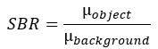
   1. Compute mean object intensity across all segmented ROIs in the marker's intended detection channel.
   2. Define background intensity as the mean intensity of all pixels outside ROIs in the same field of view, excluding zero-valued padding or out-of-bounds pixels.
      Calculate SBR as:
      
   3. Visualize SBR distributions with violin plots, showing per-object values as points (or per-field values where indicated).
6. Bleed-through quantification
   1. For each non-intended channel, compute bleed-through (%) using the same ROIs from the mask in step 12.2:
      
   2. NOTE: diagonal entries equal 100%, since in the intended channel of a single-stain image, the numerator and denominator are identical (true marker signal measured in its own channel).

Results

Two fundamental challenges faced by immunofluorescence imaging techniques are the non-specific binding of fluorophore-conjugated antibody probes and tissue autofluorescence. This protocol is designed to help distinguish a true signal from background to optimize multiplexed immunofluorescence techniques.

Heparin blocking reduces non-specific fluorophore binding while preserving signal

Discussion

Spectral IBEX, an adaptation of the IBEX protocol, successfully addresses two key issues in immunofluorescence imaging: non-specific binding and autofluorescence. Treating highly eosinophilic tissues with heparin and using spectral unmixing to eliminate autofluorescence and spectral overlap between channels significantly increased the detection of true signal above background. Capturing all markers in a single pass reduces acquisition time, which may increase the rate of IBEX cycling. While conventional confocal acquisit...

Materials

List of materials used in this article

Name	Company	Catalog Number	Comments
2N sulfuric acid (H2SO4) solution	N/A	N/A	Whatever is available/used in the lab
500 mL beaker	N/A	N/A	Whatever is available/used in the lab
6-well plate	N/A	N/A	Whatever is available/used in the lab
Bcl-6 - Alexa Fluor 647	BD Biosciences	561525	Dilution factor 1:100
BD Cytofix/Cytoperm Fixation/Permeabilization Kit	BD Biosciences	554722
Benchtop dissection microscope	N/A	N/A	Whatever is available/used in the lab
Bovine Serum Albumin (BSA)	SIGMA-ALDRICH	A4503
CD11c - Alexa Fluor 700	BD Biosciences	561352	Dilution factor 1:100
CD138/Syndecan-1 - PE	BioLegend	356503	Dilution factor 1:200
CD20 - Alexa Fluor 488	Invitrogen	53020282	Dilution factor 1:100
CD21 - Alexa Fluor 532	NovusBio	NBP2-60733AF532	Dilution factor 1:100
CD23 - PE	BioLegend	338507	Dilution factor 1:200
CD3 - iFluor 594	AAT Bioquest	100320C0	Dilution factor 1:100
CD31 - Alexa Fluor 700	BioLegend	303134	Dilution factor 1:100
CD34 - iFluor 594	AAT Bioquest	103400C0	Dilution factor 1:100
CD38 - Alexa Fluor 700	BioLegend	303523	Dilution factor 1:100
CD4 - Alexa Fluor 647	BioLegend	300520	Dilution factor 1:100
CD45 - Alexa Fluor 532	ThermoFisher Scientific	58045942	Dilution factor 1:100
CD54/ICAM-1 - Alexa Fluor 647	BioLegend	353113	Dilution factor 1:100
Chrome Alum-Gelatin Adhesive	Newcomer Supply	1033A
Cryomold	Fisher Scientific	NC9511236	Also, Catalog No.50-465-347 for bigger samples
DAPI calibration slide	Agar Scientific	AG2273
DAPI solution, 1 mg/mL	ThermoFisher Scientific	62248	Dilution factor 1:3000
E-cadherin/CD324 - Alexa Fluor 647	BioLegend	147307	Dilution factor 1:100
EpCAM/CD326 - Alexa Fluor 594	BioLegend	324228	Dilution factor 1:100
Eppendorf/falcon tubes	N/A	N/A	Whatever is available/used in the lab
Fluoromount-G	SouthernBiotech	0100-01
Forceps	N/A	N/A	Whatever is available/used in the lab
FoxP3 - eFluor 660	ThermoFisher Scientific	50577382	Dilution factor 1:100
Frosted end microscope slides	ChemScience	GEW45-2575-W
GL7 - Alexa Fluor 488	ThermoFisher Scientific	53590282	Dilution factor 1:100
Heparin sodium salt	SIGMA-ALDRICH	H3393	10KU
HLA-DR - PE	NovusBio	NB100-77855PE	Dilution factor 1:200
Human TruStain FcX (Fc Receptor Blocking Solution)	BioLegend	422302	Dilution factor 1:100
Humidity chamber	N/A	N/A	Whatever is available/used in the lab
Ice bucket with lid	N/A	N/A	Whatever is available/used in the lab
IgD - Alexa Fluor 488	BioLegend	348215	Dilution factor 1:100
IL4Ra/CD124 - PE	BioLegend	144803	Dilution factor 1:200
Imaris File Converter	OXFORD instruments	N/A	Coverting any image file format to .ims format (https://imaris.oxinst.com/microscopy-imaging-software-free-trial#file-converter)
Isopentane (2-Methylbutane)	N/A	N/A	Whatever is available/used in the lab
Ki-67 - Alexa Fluor 488	BD Biosciences	558616	Dilution factor 1:100
Kimberly-Clark Professional Kimtech Science Kimwipes Delicate Task Wipers, 1-Ply	Kimtech Science	06-666
Large (i.e., 25 cm long) forceps	N/A	N/A	Whatever is available/used in the lab
Liquid Nitrogen	N/A	N/A	Whatever is available/used in the lab
Lithium borohydride (LiBH4)	SIGMA-ALDRICH	222356
MECA-79 - Alexa Fluor 488	Invitrogen	53603680	Dilution factor 1:100
Microscope Slide Cover Glass No.1 22x50 mm	Fisher Scientific	12-542A
Milli-Q water	N/A	N/A	Whatever is available/used in the lab
MUC2 - Alexa Fluor 488	NovusBio	NB120-11197AF488	Dilution factor 1:100
Nunc Lab-Tek Chambered Coverglass	ThermoFisher Scientific	155380
PAP pen	abcam	AB2601
Phosphate buffered saline (PBS) solution	N/A	N/A	Whatever is available/used in the lab
Scalpel	N/A	N/A	Whatever is available/used in the lab
SimpleITK Imaris Extensions	N/A	N/A	Software used to align images from different rounds (https://github.com/niaid/imaris_extensions)
Sucrose	SIGMA-ALDRICH	S0389
Tissue-Tek O.C.T. Compound	Sakura Finetek USA	4583
Triton X-100	SIGMA-ALDRICH	X100
Zeiss LSM 980	ZEISS Microscopy	N/A	The imaging system used in this study
Zen Blue	ZEISS Microscopy	N/A	The software used for post acquisition image processing

References

- Hagios, C., Lochter, A., Bissell, M. J. Tissue architecture: The ultimate regulator of epithelial function. Philosoph Trans Royal Soc B: Biol Sci. 353 (1370), (1998).
- Mincarelli, L., Lister, A., Lipscombe, J., Macaulay, I. C. Defining Cell Identity with Single-Cell Omics. Proteomics. 18 (18), (2018).
- Macaulay, I. C., Voet, T. Single Cell Genomics: Advances and Future Perspectives. PLoS Genet. 10 (1), (2014).
- de Vries, N. L., Mahfouz, A., Koning, F., de Miranda, N. F. C. C. Unraveling the Complexity of the Cancer Microenvironment With Multidimensional Genomic and Cytometric Technologies. Front Oncol. , 10(2020).
- van Dam, S., Baars, M. J. D., Vercoulen, Y. Multiplex Tissue Imaging: Spatial Revelations in the Tumor Microenvironment. Cancers. 14 (13), (2022).
- Bressan, D., Battistoni, G., Hannon, G. J. The dawn of spatial omics. Science. 381 (6657), (2023).
- Williams, C. G., Lee, H. J., Asatsuma, T., Vento-Tormo, R., Haque, A. An introduction to spatial transcriptomics for biomedical research. Gen Med. 14 (1), (2022).
- Ståhl, P. L., et al. Visualization and analysis of gene expression in tissue sections by spatial transcriptomics. Science. 353 (6294), (2016).
- Pascal, L. E., et al. Correlation of mRNA and protein levels: Cell type-specific gene expression of cluster designation antigens in the prostate. BMC Genom. 9, (2008).
- Patel, S. S., Rodig, S. J. Overview of Tissue Imaging Methods. Methods Mol Biol. 2055, (2020).
- Ohno, M., Karagiannis, P., Taniguchi, Y. Protein expression analyses at the single cell level. Molecules. 19 (9), (2014).
- Zimmermann, T., Marrison, J., Hogg, K., O’Toole, P. Clearing up the signal: Spectral imaging and linear unmixing in fluorescence microscopy. Methods Mol Biol. , 1075(2014).
- Radtke, A. J., et al. IBEX: an iterative immunolabeling and chemical bleaching method for high-content imaging of diverse tissues. Nat Protoc. 17 (2), (2022).
- Radtke, A. J., et al. IBEX: A versatile multiplex optical imaging approach for deep phenotyping and spatial analysis of cells in complex tissues. Proc Natl Aca Sci U S A. 117 (52), (2020).
- Kothurkar, A. A., et al. ’Iterative Bleaching Extends Multiplexity’ facilitates simultaneous identification of all major retinal cell types. J Cell Sci. 137 (23), (2024).
- Cohn, D. E., et al. Delineating spatial cell-cell interactions in the solid tumour microenvironment through the lens of highly multiplexed imaging. Front Immunol. 14, (2023).
- Radtke, A. J., et al. IBEX: An open and extensible method for high content multiplex imaging of diverse tissues. arXiv. , (2021).
- Radtke, A. J., et al. The IBEX Knowledge-Base: A central resource for multiplexed imaging techniques. PLoS Biol. 23 (3), e3003070(2025).
- Croce, A. C. Light and Autofluorescence, Multitasking Features in Living Organisms. Photochem. 1 (2), (2021).
- Wizenty, J., et al. Autofluorescence: A potential pitfall in immunofluorescence-based inflammation grading. J Immunol Methods. 456, (2018).
- Donaldson, J. G. Immunofluorescence Staining. Curr Protoc Cell Biol. 69 (1), 4.3.1-4.3.7 (2015).
- Sicherre, E., Favier, A. L., Riccobono, D., Nikovics, K. Non-specific binding, a limitation of the immunofluorescence method to study macrophages in situ. Genes. 12 (5), (2021).
- Monique Hartlen Histotechnology Lab Manual. , NSCC. (2022).
- Stephen Peters Frozen Section Technique. , Pathology Innovations, LLC. https://pathology-innovations.squarespace.com/frozen-section-technique (2023).
- Stringer, C., Wang, T., Michaelos, M., Pachitariu, M. Cellpose: a generalist algorithm for cellular segmentation. Nat Methods. 18 (1), (2021).
- Mayeno, A. N., Hamann, K. J., Gleich, G. J. Granule-associated flavin adenine dinucleotide (FAD) is responsible for eosinophil autofluorescence. J Leukocyte Biol. 51 (2), (1992).
- Jenvey, C. J., Stabel, J. R. Autofluorescence and Nonspecific Immunofluorescent Labeling in Frozen Bovine Intestinal Tissue Sections: Solutions for Multicolor Immunofluorescence Experiments. J Histochem Cytochem. 65 (9), (2017).
- Vlaminck, S., et al. The importance of local eosinophilia in the surgical outcome of chronic rhinosinusitis: A 3-year prospective observational study. Am J Rhinol Allergy. 28 (3), (2014).
- Skinner, B. M., Johnson, E. E. P. Nuclear morphologies: their diversity and functional relevance. Chromosoma. 126 (2), (2017).
- Duhamel, R. C., Johnson, D. A. Use of nonfat dry milk to block nonspecific nuclear and membrane staining by avidin conjugates. J Histochem Cytochem. 33 (7), (1985).
- Valnes, K., Brandtzaeg, P. Selective inhibition of nonspecific eosinophil staining or identification of eosinophilic granulocytes by paired counterstaining in immunofluorescence studies. J Histochem Cytochem. 29 (5), (1981).
- Panchuk-Voloshina, N., et al. Alexa dyes, a series of new fluorescent dyes that yield exceptionally bright, photostable conjugates. J Histochem Cytochem. 47 (9), (1999).
- Bystrom, J., Amin, K., Bishop-Bailey, D. Analysing the eosinophil cationic protein - a clue to the function of the eosinophil granulocyte. Respiratory Res. , 12(2011).
- Rahman, A. H., Tordesillas, L., Berin, M. C. Heparin reduces nonspecific eosinophil staining artifacts in mass cytometry experiments. Cyt Part A. 89 (6), (2016).
- Saitou, T., et al. Tissue intrinsic fluorescence spectra-based digital pathology of liver fibrosis by marker-controlled segmentation. Front Med. 5 (DEC), (2018).
- Acuña-Rodriguez, J. P., Mena-Vega, J. P., Argüello-Miranda, O. Live-cell fluorescence spectral imaging as a data science challenge. Biophys Rev. 14 (2), (2022).
- Constantinou, P., Dacosta, R. S., Wilson, B. C. Extending immunofluorescence detection limits in whole paraffin-embedded formalin fixed tissues using hyperspectral confocal fluorescence imaging. J Microscopy. 234 (2), (2009).
- Enninful, A., Baysoy, A., Fan, R. Unmixing for ultra-high-plex fluorescence imaging. Nat Comm. 13 (1), (2022).
- Chang, Q., et al. Imaging Mass Cytometry. Cyt Part A. 91 (2), (2017).
- Angelo, M., et al. Multiplexed ion beam imaging of human breast tumors. Nat Med. 20 (4), (2014).
- Baharlou, H., Canete, N. P., Cunningham, A. L., Harman, A. N., Patrick, E. Mass Cytometry Imaging for the Study of Human Diseases—Applications and Data Analysis Strategies. Front Immunol. 10, (2019).
- Goltsev, Y., Nolan, G. CODEX multiplexed tissue imaging. Nat Rev Immunol. 23 (10), 613-613 (2023).
- Black, S., et al. CODEX multiplexed tissue imaging with DNA-conjugated antibodies. Nat Protoc. 16 (8), (2021).
- Vorobjev, I. A., Kussanova, A., Barteneva, N. S. Development of Spectral Imaging Cytometry. Methods Mol Biol. 2635, (2023).
- Hernandez, S., et al. Multiplex Immunofluorescence Tyramide Signal Amplification for Immune Cell Profiling of Paraffin-Embedded Tumor Tissues. Front Mol Biosci. 8, (2021).
Access restricted. Please log in or start a trial to view this content.
Reprints and Permissions