Adapting Taylor Dispersion to Measure the Dispersion Coefficient of Electrolyte Solutions via an Accessible Microfluidic Setup

Summary

Here, we present a protocol to adapt the Taylor dispersion experiment to the microscale using microchannels fabricated in-house with a desktop craft cutter. The experimental platform can be used to compute the diffusion coefficient of single-species passive tracers and to visualize multispecies ion interaction and separation.

Abstract

The field of microfluidics has become increasingly prominent as it allows for rapid and precise control of fluids and particles, making it easier to synthesize compounds and separate mixtures. We perfected an accessible, repeatable microscale adaptation of the Taylor Dispersion experiment using microchannels fabricated in-house with a desktop craft cutter. The starter cost of this fast and accessible microfluidics xurography technique is approximately 300 USD, orders of magnitude lower than typical photolithography methods. Pressure-driven laminar flow from a programmable syringe pump transports an injected tracer solution downstream in the microchannel, where a digital single-lens reflex (D-SLR) camera with a macro lens captures the tracer concentration evolution over time at a fixed location. Using this experimental platform, we can compute the diffusion coefficients for single-species passive tracers under varying experimental conditions. We then extended the protocol to electrolyte mixtures, observing preliminary evidence of diffusivity changes arising from nontrivial ion-ion coupling effects. This accessible experimental method provides a practical tool for probing multispecies transport and offers insights into the complex interactions governing ionic mobility.

Introduction

In recent years, significant research efforts have been focused on investigating and developing cost-effective microfluidic devices that offer precise control over flow, particles, and solute transport. Multispecies electrolyte solutions play a critical role in a wide range of applications, from energy storage and biomedical diagnostics to environmental monitoring and water purification. Understanding how different ion species diffuse and interact in these systems is essential for optimizing performance and stability in electrochemical and transport-driven processes.

When an electrolyte solution contains ions with different diffusion coefficients, their unequal migration induces an internal electric field, even in the absence of an externally applied voltage. Faster-diffusing ions tend to separate from slower ones, momentarily creating a charge imbalance. To preserve electroneutrality, the system generates a diffusion-induced electric potential. This field slows the faster ions and accelerates the slower ones. The resulting electric potential depends on the relative ion mobilities and concentration gradients and is well described by the Nernst-Planck equations under electroneutrality constraints. Classical electrochemical models, such as the Henderson and Nernst equations, quantify this phenomenon by relating it to ion transport numbers and concentration differences¹.

Taylor dispersion analysis has long been a powerful technique to measure molecular diffusivity by observing how a solute spreads in a pressure-driven laminar flow through a straight channel^2,3. It accounts for the interplay between advection and diffusion and enables accurate inference of molecular diffusion coefficients from effective dispersion rates. This method is particularly attractive because it combines precision, minimal sample requirements, and fast data acquisition. Traditionally used for single-species tracers, recent theoretical extensions now enable its application to multispecies systems, allowing researchers to theoretically infer individual ion diffusivities based on the coupled transport behavior⁴.

However, the high cost and technical complexity of conventional microfluidic setups–often based on cleanroom-dependent photolithography–pose significant barriers to the broader adoption of this method. In this work, we present a low-cost, accessible, and reproducible adaptation of the Taylor dispersion technique, which employs microchannels fabricated via xurography with a desktop craft cutter. This approach, with a startup cost of approximately 300 USD, allows for rapid prototyping and consistent channel fabrication without the need for costly specialized facilities⁵. Using brightfield imaging via a D-SLR camera and macro lens, the protocol builds a time series of the tracer concentration evolution at a fixed capture point downstream from the injection site⁶. We demonstrate that this platform can accurately measure diffusion coefficients for single-species passive tracers and extend the method to analyze multispecies electrolyte systems. Results reveal clear signatures of diffusivity variations arising from ion-ion coupling effects. This accessible and cost-effective method offers a practical tool for investigating ionic transport phenomena in complex electrolyte mixtures. For example, the proposed experimental setup can be readily adapted to be used as a micromixer to evaluate the mixing efficiency of multispecies solutes⁷, or to design desired polymer molecular weight distributions through a computer-controlled tubular flow reactor⁸.

Protocol

1. Materials preparation

NOTE: In this report, microfluidic chips are built by cutting microchannel designs in a single layer of polyimide tape with a width w = 2.54 cm and thickness h = 100 µm, which is then sealed between two polyester sheets. The aspect ratio of the microchannel (λ = h/w) is dependent on the thickness of the polyimide; the width of the channel (w) is the only cross-sectional feature that is modifiable in this protocol.

1. Cut the polyimide tape into a 21 cm-long strip.
2. Cut two polyester rectangles of length 21 cm and width 5 cm.
   NOTE: To fabricate each 18.77 cm-long microchannel, one polyimide strip and two polyester rectangles are needed. One of the polyester rectangles is cut using the desktop craft cutter to create inlet and outlet holes, while the other is used unaltered.
3. Cut and set aside a second strip of polyimide tape of length 21 cm for the gasket creation. This length produces 32 gaskets; one gasket is needed for each microchannel.
4. Obtain the microchannel port by three-dimensional (3D)-printing on a resin printer.
   1. Print one port per microchannel. An .sdlprt file for the port is included in Supplementary File 1. Design the threads for Luer lock syringe tips to be screwed into the port for a watertight seal.
   2. 3D-print solid (no infill) directly on the build platform with no additional supports. Set layer thickness to 0.10 mm.
   3. Cure post print in a UV chamber for 15 min at 60 °C.

2. Assembly of the experimental setup

1. Fabrication of the microfluidic chip top layer.
   1. Launch the craft cutter design software.
   2. Design the microchannel top using the craft cutter design software, or by importing a design from other compatible software.
   3. Draw two circles of diameter 0.27 cm at a distance of 18.77 cm from one another: these are the flow inlet and outlet. At a distance of 2.71 cm from the inlet hole, draw a smaller tracer inlet hole of 0.15 cm diameter.
      NOTE: A .DXF template file (Supplementary File 2) is included as a reference.
   4. Attach one of the two polyester rectangles from step 1.2 to the sticky side of the cutting mat. Using 2.54 cm-wide masking tape, tape along the four sides of the perimeter.
      NOTE: As polyester sheets are uniform on both sides, they can be used with either side being "up". The masking tape is necessary to prevent any movement of the polyester while cutting. The other polyester rectangle cut in step 1.2 is used as is.
   5. Ensure the craft cutter is connected to the computer with the design software via a universal serial bus (USB) cable or Bluetooth.
   6. Load the cutting mat into the craft cutter by aligning the marked edges of the mat with the arrow markings on the cutter. Insert the blade into the carriage slot of the craft cutter.
      NOTE: Potential errors in the microchannel fabrication are primarily a result of either blade wear or misalignment. Blade wear can cause the walls of the channels to be cut roughly and unevenly. To address this issue, a different blade is used to cut each type of material to reduce rapid blade sharpness degradation. Following this principle, two blades are needed in this protocol, one for the polyester and another for the polyimide tape. If, while manufacturing channels, the walls of the channel become noticeably rougher or the negative becomes difficult to remove, the blade may need replacing. Blade misalignment may cause the blade not to penetrate the material at the correct angle, resulting in wider or narrower channels. This issue is more common in channels of smaller width but can be mitigated by designing the channel walls to be the long sides of a continuous cut rectangle, rather than separate parallel lines.
   7. On the top right of the design page on the computer monitor, click send to proceed to review materials and cut settings.
   8. Input the polyester sheet cut settings. With this setup, the recommended settings are: Blade Depth: 9, Force: 33, Passes: 1, and Speed: 1.
      NOTE: Craft cutter setting recommendations are based on the 2019 work by Taylor and Harris⁵.
   9. Click submit to submit the job to the craft cutter. The cutter begins the cutting process, which takes approximately 15 s.
   10. Wait for the blade to return to its home position. Then, remove the cutting mat by pressing the eject button.
   11. Remove the negative polyester material using tweezers. The cut polyester sheet includes three holes: flow inlet and outlet holes 18.77 cm apart, and a smaller tracer inlet hole between the first two, 2.71 cm from the inlet hole, as shown in Figure 1A.
   12. Remove all material from the cutting mat and set the chip top aside.
       NOTE: When cutting into polyester, the blade leaves a rough edge protruding slightly from the sheet on the cut side. When assembling the microfluidic chip, face this edge up (away from the polyimide) to avoid it interfering with the flow through the microchannel.
2. Cut gasket
   1. Design donut-shaped polyimide gaskets using the craft cutter design software, or by importing a design from other compatible software.
   2. Draw two concentric circles of diameters 0.52 cm and 0.24 cm, respectively.
      NOTE: A .DXF template file with 32 gaskets is included as Supplementary File 3. One gasket is needed for each port when attaching it to the microchannel.
   3. Attach polyimide tape from step 1.3 to the cutting mat, both with the sticky side up. Using 2.54 cm-wide masking tape, tape along the four sides of the perimeter.
   4. Load the cutting mat into the craft cutter by aligning the marked edges of the mat with the arrow markings on the cutter.
   5. Replace the blade used for polyester sheets with a new blade to be used exclusively to cut polyimide tape.
   6. On the top right of the design page on the computer monitor, click send to proceed to review materials and cut settings.
   7. Input the polyimide tape cut settings. With this setup, the recommended settings are: Blade Depth: 9, Force: 1, Passes: 1, and Speed: 1.
      NOTE: Craft cutter setting recommendations are based on the 2019 work by Taylor and Harris⁵.
   8. Click submit to submit the job to the craft cutter. The cutter begins the cutting process, which takes approximately 40 s.
   9. Wait for the blade to return to its home position. Then, remove the cutting mat by pressing the eject button.
3. Assembly of the top sheet, gasket, and port
   1. Place the polyester sheet cut in step 2.1 on a flat surface, protrusions facing upwards.
   2. Use tweezers to peel off one gasket from the polyimide tape cut in step 2.2 and lay it onto a 3D-printed port's flat underside. Align the port and gasket holes; to help with this, insert a syringe tip through the port and use it as guidance.
   3. Attach the port with gasket to the polyester sheet, laying flat, by aligning the port and flow inlet hole. Again, use the syringe tip to center the port to the sheet inlet hole. Hold in place for 30 s to help seal the double-sided polyimide gasket to the polyester chip top.
      NOTE: The port and top sheet should be firmly connected at this point, with the ability to lift the port and the top sheet together by picking up just the port.
   4. Apply a small amount of superglue to the perimeter of the port while pushing down on it to create a permanent watertight seal.
   5. Leave to the side for 2-3 h or use superglue activator spray and wait 10 min to ensure a watertight seal.
      NOTE: Use gloves and work in a fume hood when handling superglue.
4. Fabrication of polyimide microchannel body
   1. Design a microchannel body using the craft cutter design software, or by importing a design from other compatible software.
   2. Draw two circles of diameter 0.36 cm at a distance of 18.6 cm from one another: these correspond to the flow inlet and outlet holes of the chip top designed in 2.1.3.
   3. In between these two holes, insert a rectangle of the desired width and of length 18.77 cm. Make sure 0.05 cm of the rectangle overlaps with the inlet and outlet holes to reduce the risk of accidental tearing when removing the negative.
   4. Draw a single perpendicular 0.2 cm line positioned 17.71 cm from the flow inlet hole and 0.2 cm away from the channel on either side.
      NOTE: A .DXF template file is included as Supplementary File 4. This design is for a microchannel of length 18.77 cm and width 400 µm, as shown in Figure 1B.
   5. Attach the polyimide tape cut in step 1.1 to the cutting mat, both with the sticky side up. Using 2.54 cm-wide masking tape, tape along the four sides of the perimeter.
   6. Load the cutting mat into the craft cutter by aligning the marked edges of the mat with the arrow markings on the cutter. Keep the same blade used to cut the gaskets in step 2.2.
   7. On the top right of the design page on the computer monitor, click send to proceed to review materials and cut settings. Use the same cut settings input for the gaskets in step 2.2.7.
   8. Click submit to send the job to the craft cutter. The cutter begins the cutting process, which takes approximately 15 s.
   9. Wait for the blade to return to its home position. Then, remove the cutting mat by pressing the eject button on the craft cutter. A microchannel with visible inlet, outlet, and capture point features is now cut into the polyimide.
      NOTE: Orient the chip so that the capture point is closer to the outlet; in the design provided, it is 1.107 cm from the outlet, so that the distance between the tracer inlet hole and the capture point is 15 cm.
   10. Remove the negative polyimide material from the channel using tweezers. Depending on the width and features of the microchannel, this is a very delicate procedure better suited for high-precision tweezers.
   11. Remove all material from the cutting mat and set the microchannel aside; ensure the sticky side remains untouched.
5. Assembly of the microfluidic chip
   1. Place the polyimide tape sticky side up on a flat surface.
   2. Place the bottom polyester rectangle (with no holes) sized in step 1.2 onto the exposed polyimide tape. Center the polyimide strip within the width of the polyester.
   3. Apply downward pressure with a roller to remove any larger bubbles and inspect for debris or folds in the polyamide.
   4. Flip the polyimide tape and remove its protective cover from the underside.
   5. Align the top polyester sheet mounted with the 3D-printed port to the polyimide tape's inlet and outlet, and lay the polyester sheet on top of the polyamide.
   6. Apply downward pressure with a roller to remove any larger bubbles and inspect for debris or folds in the polyimide tape.
      NOTE: Significant debris in the channel or at the walls, along with misaligned inlet and outlet holes, impacts the laminar flow, compromising the experiment. This completes the fabrication of a microfluidic chip as shown in Figure 1C.
6. Assembly of the experimental area
   1. Syringe pump setup
      1. Fill a 0.5 mL glass syringe with deionized (DI) water. Mount the syringe onto the programmable syringe pump and press the fast-forward button until water begins to come out of the syringe tip.
      2. Cut and connect a 50 cm-long piece of polytetrafluoroethylene (PTFE) tubing (0.3048 mm ID, 0.762 mm OD) to a 27-G syringe tip of length 1.27 cm and OD 0.4064 mm. Use tweezers to insert the tubing over the syringe tip and pull down.
         NOTE: Make a small cut of approximately 1 mm to provide a wider opening area in the PTFE tubing and guide the syringe tip into it, as shown in Figure 2.
      3. Fill the syringe tip connected to the tubing with DI water so that a convex meniscus is formed at the opening.
      4. Attach the tip to the glass syringe mounted on the pump, ensuring that no air bubbles form in the syringe or syringe tip.
      5. Set the syringe pump to infuse only. Input the syringe type and size as 0.5 mL.
   2. Light panel setup
      1. Plug in the light panel and position it near the edge of the lab bench. This is the surface on which the microchannel will be taped, and the experimental run will occur.
      2. Turn the light panel on to its highest brightness mode. Ensuring consistent lighting in the area in which the experiments are conducted is vital as every change influences the camera's image capturing.
      3. Tape the microfluidic chip assembled in step 2.5 to the light panel using 2.54 cm-wide masking tape.
         NOTE: Tape the channel close enough to the edge of the lab bench so that it can be photographed with the camera setup described in step 2.6.3. In this experimental setup, such a distance is 1 cm.
   3. Camera setup
      1. Insert the secure digital (SD) card in the D-SLR camera and use a plug-in battery to power the camera. Mount a 20 mm f/2 macro lens onto the camera. Connect the camera to a remote trigger.
      2. Set up the tripod and mount the camera with the macro lens above the experiment, facing down. Use a level to ensure the macro lens is parallel to the channel region of interest.
      3. Center the camera view on the capture point cut in the polyimide tape. The camera should be at least 1 cm above the light panel so that it can capture both the capture point cut and a wide channel view. Images will be captured at a fixed location downstream from the tracer inlet location.
      4. Turn on the camera and set it to manual mode with a shutter speed of 1/100 s and ISO 800. Set the Image Quality to JPEG Fine and the Image Size to Large. Set the white balance setting to Fluorescent 2. Open the image area options and set the image area to DX (24x16). The macro lens is set to F2.6 with ×4 magnification.
      5. Program the camera using the remote trigger to take pictures every 1 s.
         NOTE: Reported camera settings are based on environmental conditions and will change based on ambient lighting, camera, lens, etc.
7. Tracer preparation
   1. Measure 0.60 g of fluorescein sodium salt powder to prepare the tracer solution. Dilute powder into 1 L of distilled water to obtain the desired dye concentration (0.6 g/L concentration).
      ​NOTE: The dye used and its concentration can be changed as needed. However, it must be verified that there is a linear relationship between the tracer's intensity and concentration. Here, this was accomplished by imaging samples using experimental conditions with varying known concentrations and channel heights. The 0.6 g/L concentration of fluorescein sodium salt was chosen to be within the range producing a linear relationship when plotting the blue channel intensity values from the full red, green, and blue (RGB) image. A photo of the complete experimental setup is shown in Figure 3. Figure 4 shows top view ( Figure 4A) and side view ( Figure 4B) diagrams of the experimental setup.

3. Experimental run

1. Setup
   1. Apply a layer of scotch tape on top of the tracer inlet hole to prevent outflow, ensuring one side is folded for ease of removal.
   2. Run the programmable syringe pump to flood the microchannel with DI water at a very slow flow rate.
      NOTE: For a microchannel of dimensions h x w x l = 100 µm x 400 µm x 18.77 cm, use volumetric flow rate 2.4 µL/min (corresponding to flow rate 0.1 cm/s).
   3. When flooding is completed after approximately 5 min, ensure no air bubbles have formed.
      NOTE: If air bubbles form and cannot be removed by simply extending the flooding time, remove deionized water and flush the microchannel with a small amount of ethanol or other fluid with low cohesion and low surface tension. Then, quickly flood the channel with deionized water again, making sure to first flush it well so that no ethanol is left.
   4. Turn off the syringe pump.
2. Initial condition
   1. Fill a 0.5 µL micropipette tip with the tracer mixed in step 2.7.
   2. Peel the tape covering from the tracer inlet hole using the folded tab. Using the corner of a low lint wipe, lightly remove DI water from the tracer inlet hole and wait 30 s to guarantee the DI water fronts stabilize.
   3. Once the time has passed, discharge the micropipette content into the inlet hole. Reseal the hole immediately by smoothing the tape over it using minimal pressure in a fluid motion.
      NOTE: This step creates the tracer initial condition. Before the experimental run can be initiated, the tracer will have to diffuse across the microchannel's cross-section.
   4. Wait for a time t_w > t_wd for the tracer bolus to diffuse across the cross-section of the microchannel.
      NOTE: Calculate the diffusion time along the channel width as t_wd = (w/2)²/κ, where κ is the tracer's molecular diffusion coefficient (cm²/s) and w/2 is half the width of the microchannel. Assuming that the tracer is injected in the middle of the channel, the furthest it will have to travel to reach a wall during this wait period is half its width. This way of computing the wait-time, t_w, is generalizable to any cross-section with an appropriate choice of characteristic length. In the representative results reported here, the wait-time is approximately t_w = 14 s for w = 400 µm, and h = 100 µm.
3. Flow
   1. Ensure the syringe pump is set to the desired volumetric flow rate.
   2. Simultaneously start the syringe pump and activate the remote trigger. Run the experiment for 5 min, taking photos at 1 frame per second.
      ​NOTE: A 2.4 µL/min volumetric flow rate corresponds to a flow rate 0.1 cm/s in a microchannel with w = 400 µm and height h = 100 µm (aspect ratio: λ = 1/4).

4. Data processing

1. Remove the memory card from the camera and download the images to a computer with the image processing software to be used for analysis.
2. Experimental data processing
   NOTE: The code files used for data processing are included in Supplementary File 5.
   1. Launch the data processing files provided. An image captured by the D-SLR camera pops up on the screen. Click and drag a rectangular area, aligning its height with the distance between the microchannel's walls.
   2. If the horizontal sides of the rectangle are not perfectly aligned with the walls of the microchannel, the image needs to be rotated. Hover the cursor over a corner of the rectangle, click and rotate it so that its horizontal walls are parallel to those of the microchannel. Press any key to continue; the photo pop-up closes and reopens after being rotated, as shown in Figure 5A.
   3. Click and drag a square area with the side length matching the distance between the microchannel's walls and centered at the capture point. This will be the region of interest for data acquisition, shown in Figure 5B; each image in the sequence will be cropped using this same region. Press any key to continue; the image pop-up will close.
   4. At each pixel of the cropped region, extract the blue channel from the full RGB image (Figure 5C) and invert it by subtracting its value from 255, the maximum color-channel value (Figure 5D).
      NOTE: Select the blue channel ('B' out of the full RGB) as it is the best at capturing fluorescein dye intensity when trying to distinguish between the channel region from the polyimide tape boundary with the lighting source being used⁶.
   5. Compute the mean inverted blue channel intensity value for the cropped region.
   6. Repeat steps 4.2.4-4.2.5 for all remaining images to extract and store the mean inverted blue channel intensity value for the cropped region in each photo. This results in a time series for the average intensity of the inverted blue channel at the capture point.
3. Extrapolated fit
   1. The built-in nonlinear curveFitter toolbox in the code takes as input the average intensity of the inverted blue channel time series produced in step 4.2.6 and produces a fit using the custom equation:
      (1)
      The code uses a nonlinear least squares approach to compute the best fit for four parameters: h₃, x₁, K, and h₄. Here, h₄ is a correction for the experimental baseline intensity measured when the microchannel is filled with DI water. Parameter K is the experimental enhanced dispersion coefficient.
      NOTE: Equation (1) is adapted from the Taylor dispersion theory prediction for the tracer concentration evolution over time^2,5,9 reported in the representative results as equation (2).

Results

 The microfluidic chip fabrication steps are shown in Figure 1. We include in Figure 2 the suggested steps to connect PTFE tubing to the syringe tip used to inject the background flow of deionized water (DI) in the microfluidic chip through the programmable syringe pump. Figure 3 includes a labeled photo of the complete experimental setup. Figure 4 includes not to scale top view (Figure 4A) and side view (Figure 4B) diagrams of the experimental setup highlighting relative microfluidic chip and camera positioning. Figure 5 reports the sequence of operations applied to the experimental images during the data processing phase of the protocol. In Figure 5A we showcase how the code aligns the microchannel horizontally (if needed), then Figure 5B shows the cropping of the square region of interest centered around the capture point and with side length set by the microchannel width, w. Figure 5C isolates the blue channel from the full RGB image in the cropped region of interest, and then finally Figure 5D shows the inverted intensity value for the blue channel of the cropped region obtained by subtracting it from 255 (the maximum intensity for each color-channel).

Figure 6 overlays the results from one experimental run (dashed) with the corresponding extrapolated fit (solid). Here, each experimental data point is the averaged inverted blue channel intensity value computed through the data processing steps shown in Figure 5. At the fixed capture point downstream from the tracer inlet, Taylor dispersion theory^2,5,9 predicts that the tracer concentration evolution over time is described by:

  (2)

where C(t) is the cross-sectionally averaged tracer concentration (g/L), which has been verified to be linearly related to the tracer's measured intensity; C₀ is the initial tracer concentration (g/L), U is the flow rate (cm/s), t is time (s), and x (cm) is the axial coordinate in the channel with respect to the tracer injection location. K is the tracer's enhanced dispersion coefficient (cm²/s) due to the interplay of advection and molecular diffusion. We input the experimental parameters and use the code's nonlinear curve-fitting application (curveFitter) to find the best fit value for K. Three experimental frames for time t = 140 s, 150 s, and 200 s are shown alongside the experimental (dashed) and fitted (solid) curves produced for one experimental run at flow rate U = 0.1 cm/s in a microchannel of length 18.77 cm and aspect ratio λ = 1/4; this corresponds to Péclet number Pe 88. Here, the tracer consists of 0.6 g/L of fluorescein sodium salt diluted in DI water with molecular diffusion coefficient reported in the literature^10,11 as κ = 5.70 x 10^-6 cm²/s. All experiments reported in this manuscript were run at a room temperature of 22 °C.

The experimental enhanced dispersion coefficient, K, can be used to benchmark the validity of our experimental setup and protocol by computing a related quantity–the dispersion factor^2,5,9,12, f. This parameter depends on the geometry of the channel and is calculated as^5,12,13:

  (3)

where κ is the tracer's molecular diffusion coefficient (cm²/s) and h/2 is the chosen characteristic length. The Péclet number is a nondimensional parameter quantifying the ratio of advective to diffusive effects, Pe = Uh/(2κ). Figure 7 shows good agreement between dispersion factor results from experimental runs in microchannels with rectangular cross-sections of three different aspect ratios and flow rates, and the theoretical dispersion factor behavior^5,12,13.

Figure 1: Microfluidic chip fabrication. (A) Design for the top polyester sheet of a 21 x 5 cm chip. Three holes are cut by the desktop craft cutter, left to right, to serve as flow inlet, tracer inlet, and flow outlet, respectively. (B) Design for an 18.77 cm polyimide microchannel with capture point 15 cm downstream from the tracer inlet. (C) Exploded view of microfluidic chip assembly, bottom to top: bottom polyester layer, polyimide microchannel layer, top polyester layer with polyimide gasket and 3D-printed port. Please click here to view a larger version of this figure.

Figure 2: Diagram showing how to connect PTFE tubing to a syringe tip. The tubing ID is 0.3048 mm, and the 27-G syringe tip OD is 0.4064 mm, so making a small cut of approximately 1 mm (left) can be helpful in providing a wider opening area to guide the syringe tip (center). Use tweezers to insert the tubing over the syringe tip and pull down (right). Please click here to view a larger version of this figure.

Figure 3: Labeled photo of the experimental setup. Left to right: A D-SLR camera with a 20 mm f/2 macro lens is mounted facing down on a tripod to capture the microchannel taped to the illuminated light panel. A 0.5 mL glass syringe connected to the microchannel through PTFE tubing is set on the programmable syringe pump. The remote trigger is used to activate the camera during the experimental runs. The micropipette is used to generate the tracer initial condition, as described in step 3.2 of the protocol. Please click here to view a larger version of this figure.

Figure 4: Diagrams of the experimental setup (not to scale). (A) Top view, left to right: programmable syringe pump mounted with a 0.5 mL glass syringe; PTFE tubing connecting syringe pump to microfluidic chip; microfluidic chip taped on a light panel 1 cm away from the edge; micropipette used to inject tracer solution through tracer inlet hole; D-SLR camera with macro lens mounted on tripod face down to frame the capture point. (B) Side view, left to right: PTFE tubing connecting syringe pump to microfluidic chip; syringe tip and 3D-printed port on microfluidic chip; micropipette used to inject tracer solution through tracer inlet hole; D-SLR camera with macro lens mounted face down 1 cm above the capture point. Please click here to view a larger version of this figure.

Figure 5: Image processing steps in the provided code (see Supplementary File 5). (A) Rotated experimental image so that the microchannel is horizontal. Scale bar: 1000 µm. (B) Square selection for the region of interest (ROI) to be cropped with side length matching the distance between microchannel walls; here, 400 µm. (C) Cropped ROI where the blue channel is selected out of the full red, green, and blue (RGB)  image. Scale bar: 200 µm. (D) Inverted blue channel for the cropped ROI. Please click here to view a larger version of this figure.

Figure 6: Cross-sectionally averaged tracer intensity vs. time at camera capture point for fluorescein tracer (dashed) overlaid with the extrapolated curve fit (solid). This trial was run with a 0.6 g/L of fluorescein sodium salt in DI water tracer, on a microchannel with length 18.77 cm and aspect ratio λ = 1/4, at flow rate 0.1 cm/s and Pe 88. The inverted blue channel intensity for three experimental frames at times 140 s (blue), 150 s (orange), and 200 s (green) is shown above the plot with brightness doubled for clarity. Please click here to view a larger version of this figure.

Figure 7: Dispersion factor vs. microchannel aspect ratio. Comparison of theoretical (blue curve) and experimental values (black data points) for the dispersion factor, f. The theoretical curve is obtained using the built-in finite element method partial differential equations solver in Wolfram Mathematica (NDSolve)¹². We show average and standard deviation of experimental data for: four trials with λ = 0.1 and flow rate 0.02 cm/s; twelve trials with λ = 0.25 and flow rates 0.05 cm/s (four), 0.1 cm/s (four), and 0.2 cm/s (four); four trials with λ = 0.5 and flow rate 0.1 cm/s. All experiments were conducted on microchannels of length 6.07 cm (with capture point 3 cm downstream from the tracer inlet); results were then benchmarked on 18.77 cm microchannels. Please click here to view a larger version of this figure.

Supplementary File 1: .sdlprt file for the port  Please click here to download this file.

Supplementary File 2: .DXF template file of the chip top layer. Please click here to download this file.

Supplementary File 3: .DXF template file of the chip gaskets. Please click here to download this file.

Supplementary File 4: .DXF template file of the chip microchannel. Please click here to download this file.

Supplementary File 5: MATLAB code files used for data processing. Please click here to download this file.

Discussion

In this report, we presented a repeatable and accessible experimental setup and protocol to adapt the Taylor dispersion experiment to the microfluidic scale. We leverage an existing xurography technique⁵ to manufacture our microchannels in-house at low cost using 3D-printing and a desktop craft cutter. The current industry standard for microchannel manufacturing involves the creation of master molds in which channels can be cast. Compared to the technique discussed in this manuscript, these methods can have significantly better channel resolution and feature size (some as small as 0.1 µm), but have the drawback of much higher overhead costs, up to tens of thousands of USD¹⁴. In addition to the initial overhead cost, any change to channel design features requires both the creation of a new master mold and the curing of new channels, increasing downtime. In contrast, the starter cost of the channel manufacturing equipment used in this report is approximately 300 USD; this is comparable to the least expensive way of producing a master mold, (such as using polydimethylsiloxane (PDMS)-based techniques, but has the advantage that changes in channel design and the printing of new channels take significantly less time while maintaining surface roughness comparable to the leading manufacturing techniques for 200 µm wide channels⁵. We are able to cut a microfluidic chip in less than 5 minutes and for less than 1 USD.

In this protocol, data is recorded at a fixed capture point downstream from the tracer inlet through brightfield imaging using a D-SLR camera mounted with a macro lens. While the protocol was developed using a solution of fluorescein sodium salt in deionized water (DI), this imaging method is applicable to other types of dye, such as food coloring, as long as there is a linear relation between the tracer's intensity and concentration. The potential range of chemicals to use can be further expanded by considering their absorption spectrum and background lighting. However, we note that some food dyes are derived from plant materials and may contain more than one chemical species; caution should be employed when selecting the food coloring to be used to avoid conflicting outcomes.

The validity of this setup and protocol was verified by computing the experimental dispersion factor, f, for varying channel aspect ratio and experimental flow rate, and comparing it to its theoretical values for microchannels of rectangular cross-sections, as shown in Figure 7. We also computed the diffusion coefficient, κ, for single-species passive tracers under these varying experimental conditions. Table 1 reports the molecular diffusion coefficient of fluorescein sodium salt obtained from this experimental investigation. Specifically, the tabulated κ-values were computed from equation (3) by using experimental fits for the enhanced dispersion coefficient, K, and theoretical values for the dispersion factor, f. We report average values for four experiments on microchannels with varying aspect ratios (λ = 0.1, 0.25, and 0.5) and flow rates (0.05, 0.1, and 0.2 cm/s). For each, we also include the relative error with respect to the theoretical value^10,11, κ = 5.70 x 10^-6 cm²/s, demonstrating the accuracy of our method. Finally, for each set of experimental parameters we report the Péclet number and the nondimensional time range defined by dividing the dimensional time t when the experimental intensity curve deviates from the baseline, by diffusion time t_d = h²/(4κ). We include the nondimensionalized experimental time range to demonstrate that our system has entered the Taylor dispersion regime and therefore can be well-approximated by a Gaussian profile¹⁵. In fact, the observation times reported in the last two columns of Table 1, are approximately 2–5 (or more) times the diffusion time t_d. 

Next, we extended the protocol to investigate multispecies ion interaction and separation. We report below our results from applying the Taylor dispersion experiment to a multispecies electrolyte solution made by mixing fluorescein sodium salt and blue food coloring in DI water. Figure 8 shows the time evolution of the inverted blue channel intensity curves at the camera capture point for three solutes: blue food coloring solution in DI water (–), fluorescein sodium salt solution in DI water (...), and mixed blue food coloring and fluorescein sodium salt solution in DI water (----). Each curve is the average of five experimental trials with one standard deviation in each direction (shading). The curves show the experiments with blue food coloring alone (–) reaching a minimum first, compared to the timescale of the maximum for the fluorescein sodium salt experiments (...). This is consistent with the fact that fluorescein sodium salt has a molecular diffusion coefficient one order of magnitude smaller than that of blue 1, the dye ingredient for the blue food coloring used¹⁶. The mixed solution experiments (----) highlight this timescale difference and the consequent ion separation visible through a concavity change in the intensity profile; the curve dips below the baseline first before turning upward and peaking above the baseline. In Figure 9 we plot the same mixed solution inverted blue channel intensity curve (----) overlaid with a curve obtained by summing the individual contributions of the blue food coloring experiments and the fluorescein sodium salt experiments (+++). The difference between the two curves underlines the effect that the ion-ion interaction has on the mixed solution intensity curve. When simply adding the two individual solute contributions, the (+++) curve presents a deeper minimum driven by the strong below-baseline contribution of the blue dye solution (shown as – in Figure 8), before the concavity changes on a longer timescale compared to the mixed solution curve (----). Finally, the sum curve shows again a higher peak above the baseline compared to the mixed curve, due to the fluorescein sodium salt solution behavior (shown as ... in Figure 8). The softer peaking along with the timescale shortening is an indication of the interaction between the blue food coloring and fluorescein sodium salt ions.

The intensity profiles in Figure 6, Figure 8, and Figure 9 exhibit skewness; this may be due to a few differences between classic Taylor dispersion theory^2,5,9 and the quantity measured in the experiments. The concentration profile predicted by equation (2) is symmetric in space, but in our experimental setup the measurement is taken at a fixed capture point downstream from the tracer injection site as a function of time. When viewed as a function of time, the resulting profile is inherently skewed. This temporal asymmetry is consistent with observations reported in previous studies, including Taylor and Harris (2019)⁵. Another possible cause of skewness is the influence of the finite area of the experimental image capture window. A possible alternative to the Gaussian fit described in equation (1), involves fitting the experimental data to the integral of the Gaussian expression in equation (2) over the finite image capture region (in x), as done in Bharadwaj, Santiago, and Mohammadi (2002)¹⁷. This contribution to skewness becomes particularly relevant when the size of the capture box is comparable to the standard deviation of the Gaussian curve; here, the length of our capture window is always at least one order of magnitude smaller than the Gaussian’s standard deviation.

This low-cost experimental method provides an accessible approach to the Taylor dispersion experiment at the microscale. The most delicate step in the protocol is the manufacturing and removal of the microchannel negative. During the manufacturing process, extra care must be taken to ensure the channel is secure before cutting to prevent miscuts. When removing the negative, ensure no material is left behind and avoid any contact with the channel sidewalls, which need to be smooth, parallel, and straight to ensure reliable experimental outcomes. A limitation of this method is the inherent xurography resolution limit. In this manuscript, the most difficult channels to produce are those with width w = 200 μm (and aspect ratio λ = 0.5), which pushed against the limit of the craft cutter resolution⁵. The primary cause of error is the stepper motor employed by the craft cutter, which moves the blades in defined step increments based on mechanical gears. When designs require cuts to be in between the defined step increment, greater error is introduced. In-depth work identifying the resolution limits of this xurography method is available in the literature⁵.

This experimental procedure provides a simple way to compute the enhanced dispersion factor, K, and molecular diffusion coefficient, κ, of single-species passive tracers. Additionally, the protocol offers a straightforward way of visualizing the interaction and separation dynamics between ion species. Given the accessibility and versatility of the platform, this method is suitable for analyzing the dynamics between ion species and further understanding the complex interplay of transport phenomena and it can be readily employed in applications such as a micromixer.

					Nondimensional time
Aspect ratio, λ	Flow rate (cm/s)	Experimental κ (cm2/s)	Relative error	Péclet number (Pe)	tmin/td	tmax/td
0.1	0.02	5.813 x 10-6   ±   3.797 x 10-7	1.982 x 10-2	~ 18	~ 30	~ 52
0.25	0.05	5.333 x 10-6   ±   4.179 x 10-7	6.443 x 10-2	~ 44	~ 11	~ 27
0.25	0.1	5.655 x 10-6   ±   2.822 x 10-7	7.838 x 10-3	~ 88	~ 6	~ 16
0.25	0.2	5.978 x 10-6   ±   1.724 x 10-7	4.884 x 10-2	~ 175	~ 2	~ 10
0.5	0.1	5.444 x 10-6   ±   4.790 x 10-7	4.496 x 10-2	~ 88	~ 6	~ 16

Table 1: Experimental molecular diffusion coefficient (κ) for fluorescein sodium salt. Results are computed from equation (3) by using experimental fits for the enhanced dispersion coefficient, K, and theoretical values for the dispersion factor, f. Each row reports the average κ-value (and related standard deviation) for four experiments on microchannels with a specified aspect ratio (λ = 0.1, 0.25, or 0.5) and flow rate (0.05, 0.1, or 0.2 cm/s). For each, we include the relative error with respect to the theoretical value^10,11, κ = 5.70 x 10^-6 cm²/s, to demonstrate the accuracy of our method. Additionally, for each row we list the experimental Péclet number and the nondimensional time range defined by dividing the dimensional time t when the experimental intensity curve deviates from the baseline, by diffusion time t_d = h²/(4κ).

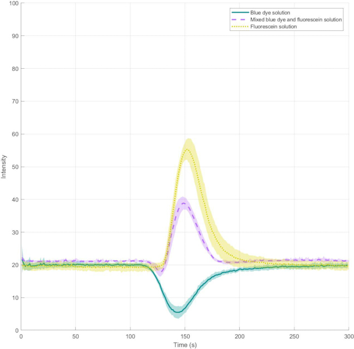
Figure 8: Time evolution of averaged inverted blue channel tracer intensity at the camera capture point for three tracers. Time evolution of averaged inverted blue channel tracer intensity at the camera capture point for three tracers: solution of blue food coloring in DI water (at concentration ratio food coloring:DI = 1:20 mL, –), solution of fluorescein sodium salt in DI water (at concentration 0.6 g/L, ...), and a mixed solution containing both blue food coloring and fluorescein sodium salt with the same concentrations as in their individual tracer experiments (----), i.e. blue food coloring:DI = 1:20 mL and 0.6 g/L of fluorescein. Each curve is the average of five experimental trials with one standard deviation in each direction (shading). Please click here to view a larger version of this figure.

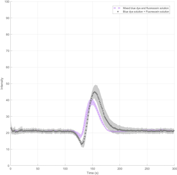
Figure 9: Time evolution of averaged inverted blue channel tracer intensity at the camera capture point for mixed solution. Time evolution of averaged inverted blue channel tracer intensity at camera capture point for mixed solution containing blue food coloring and fluorescein sodium salt (----) with blue food coloring:DI = 1:20 mL and 0.6 g/L of fluorescein, and a sum curve (+++) combining the intensity of the blue food coloring solution experiments (solid curve in Figure 8, –) and fluorescein sodium salt solution experiments (dotted curve in Figure 8, ...). The mixed curve is the average of five experimental trials with one standard deviation in each direction (shading). The standard deviation of the sum curve is calculated by taking the square root of the sum of the standard deviations squared from the experiments with each individual tracer solution. Please click here to view a larger version of this figure.

Materials

List of materials used in this article

Name	Company	Catalog Number	Comments
Adjustable volume pipette, 0.5–10 μL	MUHWA	B08TBPMKZL	Turned into table
Cameo Cutting Mat, 12 x 12 in	Silhouette America	8.19177E+11	used aphabetize function in table
Camera plug-in battery	NEEWER	B0B5WY8T96	removed 3D printed ports
Camera tripod	Vanguard	B00CCA1Y3S	added Form 2 3D printer added Form 2 3D printer
Clear Resin V5	Formlabs	https://formlabs.com/store/materials/clear-resin/	3D-printing resin
Cyanoacrylate (CA) glue accelerator	Starbond	B00BUVAZ5S	added a resin as well
D-SLR camera	Nikon	D500	added printer software
Dashboard software	Formlabs	https://formlabs.com/software/dashboard/	3D-printing software added CAD solidworks
DeIonized water	N/A	N/A	added matlab
Dimmable LED ligth panel	Kaiser Fototechnik	202455	Slimlite Plano 5000K 19.6 x 13.8 in changed the FSS lot to catalog num
Double-sided polyimide tape, 1 in x 36 yd roll	Bertech	B00HFN6E0K
Flourescein sodium salt dye - 100 g	Sigma-Aldrich	5184A17
Form 2 3D Printer	Formlabs	https://formlabs.com/3d-printers/form-2/
Glass syringe with Luer tip, 500 µL	Hamilton Company	PN: 80801
High-precision tweezers, 0.004 in wide x 0.002 in thick	McMaster Carr	ECCN: EAR99	Standard pointed tip
KimWipes	Kimtech	B0013HT2QW	4.4 x 8.4 in
Liquid pipette pipettor tips, 1000 pcs/bag	MUHWA	B07S1WJCHP	1 needed per experimental trial
Macro lens 20 mm f/2	Mitakon Zhongyi	B075JRGWW1
Masking tape, 0.70 in x 54.6 yd	Scotch Brand	B00347A8E4
MATLAB software, edition 2023b	Mathworks	https://www.mathworks.com/products/matlab.html
Medium CA Glue, 2 oz.	Starbond	126150047	Premium Cyanoacrylate Super Glue
Memory Card, 64 GB	San Disk	‎B09X7C7NCZ
Neon assorted food colors & egg dye, 1.5 fl oz	McCormick & Company, Inc.	B09PFV6275	Pink, green, and blue. Only 1 vial of blue food coloring needed. Blue food coloring ingredients: water, propylene glycol, FD&C blue 1, propylparaben (preservative).
Precision balance	Sartorius Lab Instruments	BCE224 - 1S	Entris® II Essential Line. Used to weigh fluorescein sodium salt powder for tracer mixing.
PTFE microtubing, 0.012" ID x 0.030" OD	Cole Parer	mp-00060882	Microbore transfer tubing. Minimum needed: 50 cm.
Remote programmable trigger	Pixel Pro	TW-283DC0/DC2
Scissors	Amazon	B01BRGUAT6
Scotch tape	Scotch Brand	B01C5IHGJW
Silhouette Cameo 4 Craft Cutter	Silhouette America	8.19177E+11
Silhouette Cameo AutoBlade (Type B)	Silhouette America	8.19177E+11	2 needed
Silhouette Studio Basic Edition software version 4.5	Silhouette America	https://www.silhouetteamerica.com/silhouette-studio	If importing the .DXF template files provided as part of the Supplementary Files in this software version, first set the software import settings to read the file size 'as is' by clicking: Edit > Preferences > Import > DXF > Open > As-is.
Soft rubber brayer, 4.75 x 1.75 x 6.62 in	Speedball	B003IFY622
SOLIDWORKS software, Education Edition	SOLIDWORKS	https://www.solidworks.com/solution/job-functions/educators
Standard infuse/withdraw 11 elite syringe pump	Harvard Apparatus	70-4504
Syringe tip with Luer lock, tip size: 0.5 in, 27 Gauge, Clear	Metcal	B00F4B9W40	2 needed
Ultra clear polyester sheets, 12 x 12 x 0.007 in	Grafix	B001K7Q6Z0

References

- Deen, W. M. Analysis of Transport Phenomena. , Oxford University Press. New York. (1998).
- Taylor, G. I. Dispersion of soluble matter in solvent flowing slowly through a tube. Proc R Soc Lond A. 219 (1137), 186-203 (1953).
- Bello, M. S., Rezzonico, R., Righetti, P. G. Use of Taylor-Aris dispersion for measurement of a solute diffusion coefficient in thin capillaries. Science. 266 (5186), 773-776 (1994).
- Ding, L. Shear dispersion of multispecies electrolyte solutions in the channel domain. J Fluid Mech. 970, A27(2023).
- Taylor, A. W., Harris, D. M. Optimized commercial desktop cutter technique for rapid-prototyping of microfluidic devices and application to Taylor dispersion. Rev Sci Instrum. 90 (11), 116102(2019).
- Lee, G., Luner, A., Marzuola, J., Harris, D. M. Dispersion control in pressure-driven flow through bowed rectangular microchannels. Microfluid Nanofluidics. 25, 1-11 (2021).
- Stroock, A. D., Dertinger, S. K. W., Ajdari, A., Mezic, I., Stone, H. A., Whitesides, G. M. Chaotic mixer for microchannels. Science. 295 (5555), 647-651 (2002).
- Walsh, D. J., Schinski, D. A., Schneider, R. A., Guironnet, D. General route to design polymer molecular weight distributions through flow chemistry. Nat Commun. 11 (1), 3094(2020).
- Aris, R. On the dispersion of a solute in a fluid flowing through a tube. Proc R Soc Lond A Math Phys Sci. 235 (1200), 67-77 (1956).
- Aminian, M., Bernardi, F., Camassa, R., Harris, D. M., McLaughlin, R. M. How boundaries shape chemical delivery in microfluidics. Science. 354, 1252-1256 (2016).
- Aminian, M., Bernardi, F., Camassa, R., Harris, D. M., McLaughlin, R. M. The diffusion of passive tracers in laminar shear flow. J Vis Exp. (135), e57205(2018).
- Dutta, D., Ramachandran, A., Leighton, D. T. Effect of channel geometry on solute dispersion in pressure-driven microfluidic systems. Microfluid Nanofluidics. 2, 275-290 (2006).
- Bontoux, N., Pépin, A., Chen, Y., Ajdari, A., Stone, H. A. Experimental characterization of hydrodynamic dispersion in shallow microchannels. Lab Chip. 6 (7), 930-935 (2006).
- Todd, D., Krasnogor, N. Homebrew photolithography for the rapid and low-cost,"Do It Yourself" prototyping of microfluidic devices. ACS Omega. 8 (38), 35393-35409 (2023).
- Chatwin, P. C. The approach to normality of the concentration distribution of a solute in a solvent flowing along a straight pipe. J Fluid Mech. 43 (2), 321-352 (1970).
- Gimadutdinova, L., Ziyatdinova, G., Davletshin, R. Selective voltammetric sensor for the simultaneous quantification of Tartrazine and Brilliant Blue FCF. Sensors (Basel). 23 (3), 1094(2023).
- Bharadwaj, R., Santiago, J. G., Mohammadi, B. Design and optimization of on-chip capillary electrophoresis. Electrophoresis. 23 (16), 2729-2744 (2002).
Reprints and Permissions