Using Solution NMR to Characterize Biomolecular Condensates Under Biphasic Conditions

Summary

Here we present protocols for NMR methodologies, REstricted DIFfusion of INvisible speciEs (REDIFINE) and CONdensate DEtectioN by SEmi-solid Magnetization Transfer (CONDENSE-MT) that enable label-free, quantitative characterization of biomolecular condensates under biphasic conditions, revealing molecular partitioning, exchange dynamics, condensate hydration, and droplet structure without sedimentation or labeling.

Abstract

Biomolecular condensates formed through liquid–liquid phase separation (LLPS) organize the intracellular environment and regulate diverse biochemical processes. Despite their importance, probing condensate composition, exchange dynamics, and internal organization remains challenging, particularly without external tags. Nuclear magnetic resonance (NMR) spectroscopy can provide a unique label-free window into these mesoscale assemblies, capturing both molecular motion and environmental heterogeneity. Two complementary NMR methodologies enable a comprehensive characterization of condensates directly within their biphasic state. For condensates which are dynamic enough to be observable by NMR, the diffusion-exchange approach, REstricted DIffusion of INvisible speciEs abbreviated as REDIFINE, utilizes the diffusion contrast with chemical exchange to quantify the fraction of molecules partitioned between condensed and dilute phases, determine droplet size and interface permeability, and extract molecular exchange rates across the phase boundary. For more rigid condensates that are NMR invisible, the water-detected semi-solid magnetization-transfer method, CONdensate DEtectioN by SEmi-solid Magnetization Transfer, or in short CONDENSE-MT, exploits the relaxation contrast and proton exchange between condensed biomolecules and dilute phase solvent to monitor condensates onto the bulk water protons, providing access to relative partitioning, molecular tumbling rates, hydration dynamics, and bound-water content. Together, these approaches deliver a multidimensional, quantitative view of condensate structure and dynamics under near-native biphasic conditions without fluorescent or detection tags. Their integration expands the NMR toolbox for studying biomolecular phase separation and establishes a foundation for connecting condensate physicochemical properties with their biological function and pathological misregulation.

Introduction

Cells achieve their extraordinary spatial and temporal organization by compartmentalizing biochemical reactions^1,2,3. In addition to membrane-bound organelles, many crucial cellular processes occur within membraneless compartments formed by liquid–liquid phase separation (LLPS) of proteins and nucleic acids⁴. These dynamic assemblies, often referred to as biomolecular condensates, include the nucleolus, stress granules, nuclear speckles, and processing bodies, which play essential roles in, e.g., RNA metabolism, transcription regulation, or signal transduction^5,6. Their ability to form, dissolve, and exchange components in response to environmental cues provides cells with a versatile mechanism for organizing biochemical activities without relying on lipid membranes.

A large subset of biomolecular condensates arises from RNA-binding proteins (RBPs) that contain intrinsically disordered regions (IDRs) and RNA-binding domains (RBDs)^7,8. These proteins can phase separate either alone or in complex with RNA, giving rise to condensates with diverse material properties and biological functions. For example, the SARS-CoV-2 nucleocapsid protein (N) forms RNA-dependent biomolecular condensates⁹ implicated in viral genome packaging and assembly, while the polypyrimidine tract-binding protein 1 (PTBP1) forms nuclear condensates that contribute to gene silencing¹⁰. Further, proteins such as FUS and DDX4 undergo LLPS driven by their disordered regions, influencing RNA metabolism and stress granule formation^11,12. Dysregulation of these processes is linked to neurodegenerative diseases such as amyotrophic lateral sclerosis (ALS) and frontotemporal dementia, where aberrant phase transitions can lead to aggregation and loss of function¹³.

Condensation is not limited to proteins and protein–RNA complexes. RNA alone can undergo LLPS, particularly in the context of repeat-expansion sequences associated with several neurodegenerative disorders^14,15. Trinucleotide and hexanucleotide repeat expansions, such as CAG in Huntington’s disease or CUG in myotonic dystrophy, can form droplet-like condensates both in vitro and in cells¹⁴. Understanding the physical basis of RNA condensation, as well as how it differs from protein- and protein–RNA-driven condensates, is crucial for elucidating the molecular mechanisms underlying repeat-expansion diseases.

Despite their biological importance, quantitative and label-free characterization of biomolecular condensates remains a formidable challenge¹⁶. Conventional fluorescence microscopy and spectroscopy techniques rely on external labels, which can perturb biomolecule structure, dynamics, or phase behavior^17,18. Moreover, some condensates are NMR-invisible due to restricted molecular motion and broad line shapes, limiting the information accessible by traditional NMR approaches. Consequently, there is an urgent need for experimental strategies that can probe condensates directly in their biphasic, native-like state, without labeling. Given the important role of the droplet phase boundary in exchange processes and condensate maturation, it is equally important to stabilize biomolecular droplets within a given sample volume, thereby preventing sedimentation of the dense phase. This can be readily achieved using the cytoskeleton-mimicking agarose hydrogels.

Recent developments in NMR-based methodologies provide such a solution. The REDIFINE (REstricted DIffusion of INvisible speciEs) approach¹⁹ combines diffusion NMR with chemical exchange analysis to quantify molecular partitioning, exchange kinetics, and droplet size in protein and protein–RNA condensates. Complementarily, the CONDENSE-MT (CONdensate DEtectioN by SEmi-solid Magnetization Transfer) technique²⁰ detects NMR-invisible condensates via water magnetization transfer, allowing quantification of the amount of condensed matter at given conditions and further revealing hydration dynamics and molecular tumbling rates within the condensate. Together, these methods enable label-free, non-invasive investigations of diverse condensate types, protein-only, protein–RNA, and RNA-only condensates under equilibrium biphasic conditions. By expanding the NMR toolbox, they open the door to systematic, quantitative exploration of condensate structure, dynamics, and their connections to biological function and disease.

Protocol

1. Sample preparation

1. Buffer choice: Use tested buffers in which the biomolecules are most stable. 
   NOTE: NMR signals are typically stronger at lower pH. As a technical requirement, add 5% D₂O as a field lock to all NMR samples (final v/v).
2. Stabilize the biphasic sample, using a cytoskeleton-mimicking agarose hydrogel as medium. Weigh agarose powder to prepare a 1.5% (w/v) agarose stock in the same buffer. Use regular agarose as a cheaper alternative for biomolecular condensates formed by intrinsically disordered proteins (IDPs) and RNAs that can withstand higher temperatures. Use low-melting agarose when preparing delicate condensates involving proteins that contain folded domains¹⁹.
3. Preparation of agarose stock: Heat up the suspension to ca. 80 °C for 10 min and fully dissolve the agarose by mixing or vortexing.
   CAUTION: Molten agarose is hot and can burn; handle with heat-resistant gloves.
   NOTE: Keep the molten agarose warm (e.g., 55 °C for regular agarose and 37 °C for low-melting agarose) in a water bath to remain liquid prior to mixing with the biological sample. 
   Molten agarose can be kept warm for several tens of minutes^19,21.
4. Prepare final biphasic sample:
   1. To prepare a biphasic sample stabilized by agarose hydrogel, mix protein (and/or RNA) stocks with respective warm agarose buffer in a 1.5 ml microcentrifuge tube.
      NOTE: Final protein/RNA concentration is typically 50-500 µM to be suitable for NMR detection.
   2. Immediately transfer the mixture into a 3 mm NMR tube using a long glass pipette. Allow agarose to solidify shortly after transfer.
      NOTE: Without agarose, the biphasic sample sediments over time, complicating NMR data acquisition and analysis because the sample physically changes at the time scale of the experiment.
5. Perform visual inspection: Inspect the sample visually. If phase separation occurs, the sample appears immediately turbid and remains like that. This indicates that the biphasic sample has been successfully stabilized in agarose.
6. When intending to run CONDENSE-MT, prepare an additional agarose reference sample by doing the same steps, just omitting the addition of the biomolecule. Add the buffer instead to yield the same sample volume. Prepare this sample only after preparing the condensate sample and measuring all the data on it to ensure that the agarose reference sample is not incubated for a longer time.

2. Recording REDIFINE experiments

1. Lock, shim, match, and tune the ¹H channel as usual. Calibrate the 90° pulse length on ¹H using your general procedure.
2. Record a 1D water-suppressed spectrum. Ideally strong biomolecular signal is observed (Supplementary Figure 1A).
   1. If no or very little signal is observed, assume that the condensed protein/RNA is not NMR-observable and that partitioning into the condensed phase is high. In this case, do not proceed REDIFINE as this methodology relies on an observable biomolecular signal.
   2. In this situation, in principle CONDENSE-MT experiments should work very well, so jump immediately to Step 4 (Recording CONDENSE-MT experiments).
3. Load the conventional Diffusion Ordered Spectroscopy (DOSY) experiment that relies on a conventional 2D Stimulated-Echo procedure using bipolar gradients (Bruker pulse sequence: stebpgp1s19). Consult the Bruker DOSY and Diffusion user manuals for more details.
4. Set P0, P1 and P27 to the calibrated 90° pulse length. Set as a rule of thumb, NS to 32 scans, DS to 16, TD1 to 16, and adjust TD2 and SW2 to result in acquisition time AQ of 80-100 ms. Set d1 to 1.5 s.
   NOTE: Gradients should be properly calibrated.
5. Optimize Watergate d19 delay as usual according to your magnetic field, to yield maximum excitation at aromatics (ca. 7 ppm) or aliphatics (ca. 1 ppm). Set d20 to 75 ms. The choice of p30 will depend on the protein/RNA size. For proteins >20 kDa, use 5 ms; for smaller proteins, use 3.5 ms as a rule of thumb.
6. Record a DOSY experiment by the command: ‘xau dosy 2 95 16 l y y’ which arrays the diffusion gradient strength from 2 to 95 % in 16 steps, in a linear fashion.
   1. Ideally, one should observe the initial decay of the signal stemming from the dilute phase, while the decay of the condensed phase signal should plateau (Figure 1A and Supplementary Figure 1B).
7. To continue acquiring data for the full REDIFINE set, create 9 new stebpgp1s19 by copying the parameters from the initial one that you just ran. In every consecutive experiment, change only the d20 diffusion delay in variable steps to span the range from 100–1000 ms (i.e., 100, 150, 200, 250, 300, 400, 500, 700, 1,000 ms).
8. Run each one of these experiments by the command ‘xau dosy 2 95 16 l y n’. The last “n” ensures that the receiver gain is preserved throughout the 10 experiments.

3. Processing REDIFINE datasets and visualizing the results

1. Process every experiment (10 in total) in the following manner: 
   1. Set qsine of SSB 2 as window function, extract 5^th slice using qsin;fp, phase the 1D and save the phasing parameters to the 2D dataset.
   2. Then process 2D with xf2, do baseline correction abs2, and extract these 16 slices with split2D (further inputs in the pop-up window: r – 16 – 11). This will extract 16 spectra acquired using different gradient strengths and save them as 1D processed experiments from 11 to 26 within the same dataset.
   3. Repeat the same for the remaining 9 experiments. Sometimes it is crucial to check at least the first 4-5 slices to ensure the phasing and baseline correction are correct. If needed, correct manually – good phasing and baseline are prerequisites for proper quantification (Figure 1B).
2. Use the provided Matlab code LLPS_REDIFINE_fit for the analysis (Supplementary Figure 2A). In the code, adjust according to your experiments the following: ‘Delta’ (diffusion times d20), ‘P.d’ (total gradient duration 2*p30), exp(1,:) to exp(10,:) based on the # of experiments you ran. Then set P.g according to your probe gradient strengths (accessible at TopSpin experiment folder under file “difflist”).
3. Adjust the ‘folder’ and ‘path’ based on your data location. Run the code until line 40. This will give you the 1D slice – from here, choose the integration regions; these should encompass aromatics or aliphatics, and choose the region as narrow as possible, not to account for different molecular groups such as amides.
4. Input the integration boundaries in points in variables ‘left’ and ‘right’ accordingly (Supplementary Figure 2A). This is to integrate the data for the quantitative analysis (Figure 1C). Pick the matrix name according to your sample, date of run, and some experimental specifics.
5. Run the whole code. In ‘fit0’, you can choose the starting parameters that the optimization function will use to initiate the minimization. Start with the default values, and then if convergence is not achieved, change the second fit0 value (population in the condensed phase) in steps of 0.1 from 0.1 to 1.
   NOTE: Sometimes the dataset has several local minima, and one needs to vary the starting parameters extensively in order to start converging to the more global minimum.
6. When satisfactory fitting was achieved, the fitting values will be written within the figure (Figure 1D and Supplementary Figure 2B) and can be accessed in the variable ‘fit’. Further plot these parameters as a statistics plot for better visualization. 

4. Recording CONDENSE-MT experiments

NOTE: The goal of the experiment is to indirectly detect the condensates by their observation on the solvent water signal via proton exchange²⁰. In the CONDENSE-MT experiment, a fingerprint MT profile is acquired and analyzed (Figure 2A)²⁰. 

1. Record your favorite 1D water-suppressed spectrum. If very little signal is observed, it is very likely that the CONDENSE-MT experiment will work very well.
2. Quantitative CONDENSE-MT analysis requires previous determination of the R1 rate of water. Determine the R₁ rate via T₁ inversion recovery. Copy the provided pulse sequence, Bruker parameter set, and the vd list to the respective folders. Load the parameterset “T1_inversion_recovery” and adjust powers and frequencies to your NMR spectrometer (according to “edprosol”).
   1. Calibrate the 1H 90° pulse (p1), set NS to 2, DS to 0, d1 to 20 s, SW to 10 ppm, TD2 to 16k, and TD1 to 24 (of the length of your adjusted vd list). Enable a weak gradient along Z (GPZ0 = 0.1 %) to avoid radiation damping effects.
3. For the CONDENSE-MT experiment,
   1. Copy the provided Bruker parameter set, sequence, and the frequency list to the Bruker-specific folders, load the parameter set “CONDENSE-MT”, and adjust the frequencies and powers according to your spectrometer.
   2. Set P1 to the calibrated 90° pulse length and P4 to 1 µs for the excitation pulse to avoid radiation damping. Set NS to 2, DS to 16, d1 to 4 s, SW2 to 20 ppm, TD2 to 8k, TD1 to the length of the frequency list (typically 46). Set SPNAM10 to Squa100.1000 and its duration p10 to 5 s.
   3. Find the SP10 power to yield 100 Hz irradiation (command ‘pulse 100 Hz’ will calculate your power in both watts and dB). Adjust the SP10 power of irradiation pulse accordingly and run this pseudo-2D experiment using the ‘zg’ command.
      NOTE: The experiment will use the provided frequency list that spans the irradiation offsets from on-resonance with water to very far off-resonance (100000 Hz) to detect the water signal at different irradiation offsets (Figure 2B). A plot of water integrals (ensure proper phasing of the spectra; Figure 2C) with respect to the irradiation offset yields the CONDENSE-MT profile shown in Figure 2A.
4. Create 7 new experiments and in each consecutive one, increase only the power of irradiation to cover the range from 170 Hz to 1000 Hz (i.e., 170, 250, 330, 500, 650, 780, 1,000 Hz). In every experiment, use the command from the previous point. For every saturation power, the whole offset list will be acquired (Figure 2D).
   NOTE: CONDENSE-MT fitting requires the reference data acquired on the agarose-only sample (medium without biomolecular condensates). Ensure the same time interval between sample preparation and data acquisition, and acquire the same dataset of 8 experiments on an agarose reference sample. This is to ensure that both the agarose reference and the biphasic sample were incubated for the same amount of time.

5. Processing CONDENSE-MT datasets and visualizing the results

1. Process every CONDENSE-MT experiment (8 in total, Supplementary Figure 3A) in the following manner.
   1. Set qsine of SSB 2 as the window function, extract the 46^th slice using qsin;fp, phase the water peak in 1D, and save the phasing parameters to the 2D dataset, then process 2D with xf2, and extract these 46 slices with split2D (further inputs in the pop-up window: r – 46 – 11).
      NOTE: This will extract 46 1D-spectra acquired using different irradiation offsets and save them as 1D processed experiments from 11 to 56 within the same dataset (Supplementary Figure 3A, shown for the 1000 Hz CONDENSE-MT experiment).
   2. Repeat the same for the remaining 7 experiments. Check several slices from each experiment to ensure the phasing and baseline are correct (Figure 2C). If needed, correct manually – good phasing and baseline are prerequisites for proper quantification!
2. Repeat the same steps on data acquired using agarose reference sample and for the inversion recovery experiments, extracting the 24th slice for phasing and using split2D (r – 24 – 11).
3. Fit the acquired data using the provided Matlab code. Follow the specific instructions in the script.
4. Perform the fitting analysis first for the agarose reference sample to obtain the background parameters in the absence of condensates. The read_CONDENSE_MT_data code first reads the processed NMR data and integrates the water resonance signal in the 1D slices generated by the split2D command (Supplementary Figure 3B).
5. Set the integration boundaries individually; a reference 1D spectrum will be plotted in Matlab to assess the integration boundaries (Supplementary Figure 3C). The code will further normalize the data and fit the normalized integrals of water as a function of irradiation offset and power to the CONDENSE-MT model²⁰. The read_CONDENSE_MT_data will store the normalized integrals in the variable integral_water_real_all, which is then used for subsequent fitting.
6. Determine the R₁ relaxation rate of water in the presence of agarose or condensates before fitting the CONDENSE-MT data.
   NOTE: Fitting the water inversion recovery experiment can be done within the first section of the CONDENSE-MT_full Matlab script (or the CONDENSE_MT_referenceMTpool script in case of the agarose reference data). The file name and path of the experiment, as well as the experiment ID for the experiment, can be entered to run the Inversion_Recovery Matlab script (Supplementary Figure 4A, section 1). If required, the number of 1D slices and the integration boundaries can be adjusted in this script; the latter depends on the processing parameters used in TopSpin. This section will determine the R1 rate of water and store it in the P.R1w variable, which is required for subsequent fitting of the CONDENSE-MT data.
7. For agarose data, use the normalized integrals straightforward for fitting, using the CONDENSE_MT_referenceMTpool script (which calls the function_1MT function.
8. For condensate quantification, use the fitted parameters of agarose as an input for global fitting of the data acquired on the condensed sample (Supplementary Figure 4A). This will fix the physical properties of the agarose meshwork as constant values to the fit, allowing for quantification of the condensate-mediated, additional effect of a condensate embedded in the agarose meshwork (Figure 2E).
9. Do the condensate quantification using the CONDENSE-MT_full script, which calls the function_2MT Matlab-function. The starting parameters for computational optimization are given via fit0 (Supplementary Figure 4B). The parameter uncertainty of the fit will be calculated with the Jacobian matrix from which the variance-covariance matrix will be derived (Supplementary Figure 4B).
10. Assess the quality of the fit by the fit deviation, resembling the residual deviation of model prediction from experimental data. For further quality control, plot the fit together with experimental data (Supplementary Figure 4C).

Results

The LLPS REDIFINE protocol described here was applied to the FUS N-terminal domain (NTD). FUS NTD readily phase separates under ambient conditions at micromolar concentrations^19,21. This particular sample was prepared at a concentration of 200 µM in 30 mM HEPES buffer containing 200 mM KCl at pH 7.5, with 0.5% regular agarose. Upon phase separation, FUS NTD signals remain observable in the condensed phase (Figure 1A,B). This makes it a perfect candidate for LLPS REDIFINE to study. Namely, most LLPS-prone proteins contain long intrinsically disordered regions that usually remain observable in the condensed phase; however, in more structured proteins, this is not the case.

The REDIFINE fit (Figure 1D and Figure 3A,B) revealed multiple unique parameters for this FUS NTD sample. Specifically, it determined the diffusion coefficients in the dilute and condensed phase (D_dil and D_cond), population of protein in the condensed phase (ν_cond), average droplet size R, and interphase permeability p. Droplet size and permeability define the interphase exchange rate from the condensed to the dilute phase k_cd=3p/R, allowing us to obtain the information about exchange dynamics¹⁹.

These results can be visualized in different ways (Figure 3B). Using a spider plot, one could compare results across different conditions or samples. On the other hand, one can pictorially represent the REDIFINE parameters in the model to visualize them most effectively. Note that REDIFINE provides all these results label-free in just a couple of hours using only one sample.

As the NMR signal of FUS NTD remains detectable in the condensed phase (Figure 3C), the CONDENSE-MT will most likely not be applicable due to the lack of relaxation contrast. We recorded the CONDENSE-MT data set on FUS NTD, and indeed, no difference in the MT profile is observed between the agarose reference and FUS NTD biphasic sample (Figure 3C). This renders the CONDENSE-MT methodology inapplicable to this particular FUS NTD sample.

However, the CONDENSE-MT provides dynamic characterization of repeat-expansion RNA condensates (Figure 3C,D)²⁰. Note that CONDENSE-MT could provide multiple parameters uniquely characterizing the RNA in the condensed phase (Figure 3D), despite the fact that its signal is unobservable in conventional NMR (Figure 3C). The obtained parameters are the proton-exchange kinetics between condensate and bulk water (k_{condensate,H2O} and k_{H2O, condensate}), the T₂ relaxation rate for the condensate (T_2,condensate), reflecting the extent of dynamic arrest of the biomolecules upon condensation, and the apparent R₂ rate of bulk water (R_2,water). This last parameter is a linear combination of the tumbling rate of bulk, dilute water, and slow-tumbling, condensed water. Higher R_2,water values indicate a higher population of water in the condensate, which elevates the apparent overall water R₂ rate²⁰ (Figure 2E and Figure 3D).

DATA AND CODE AVAILABILITY

LLPS REDIFINE raw data and processing codes are available in the Zenodo repository: https://doi.org/10.5281/zenodo.15228787 . CONDENSE-MT raw data and processing codes have been deposited to Zenodo repository https://doi.org/10.5281/zenodo.15789697. MATLAB is required for the processing. They are also provided within this article (Supplementary Coding Files).

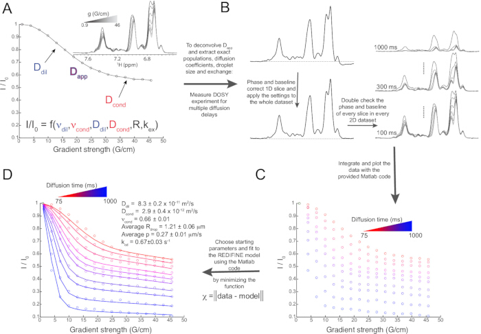
Figure 1: REDIFINE workflow. (A) Diffusion measurements yield complex biphasic diffusion decay curves in condensed samples. The resulting decay contains deconvolved parameters describing the diffusion coefficients of the species in the condensed and dilute phase, their populations, droplet size, and interphase exchange rate. (B) To decode these isolated parameters, one needs to record a pseudo-3D dataset by varying not only the gradient strength but also the diffusion delays. It is absolutely essential for quantification that every slice from these measurements be properly phased and baseline-corrected. (C) After checking the quality of the measured and processed data, these 1D slices are fed into the MATLAB code for analysis and final plotting. (D) The data are then fitted by a nonlinear programming solver. The fitting and resulting parameters are illustrated for the biphasic FUS NTD sample. Please click here to view a larger version of this figure.

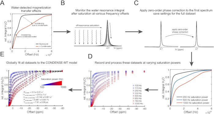
Figure 2: CONDENSE-MT workflow (A) A unique CONDENSE-MT profile observed on the water resonance illustrating the broadening due to the presence of condensed biomolecules and water. (B) Water is observed for every irradiation offset. (C) For quantification, it is essential that all spectra be phased correctly. (D) After acquiring the water resonance at different irradiation offsets, the experiment is repeated at different irradiation powers. This will yield a dataset of the relative water signal as a function of both irradiation offset and irradiation power (E). The data are then fitted by a nonlinear programming solver. The fitting and resulting parameters are illustrated for the biphasic 31xCAG RNA sample. Please click here to view a larger version of this figure.

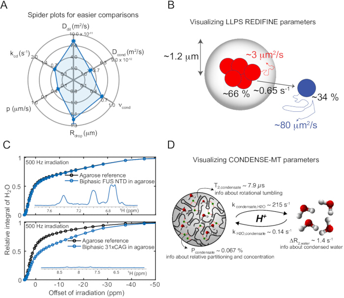
Figure 3: Presentation of REDIFINE and CONDENSE MT results. (A) Spider plot representation of REDIFINE parameters for comparative analysis across samples or conditions. (B) Schematic model illustrating REDIFINE-derived parameters, including diffusion coefficients, droplet radius, partitioning, and interphase exchange rate. (C) Comparison of CONDENSE-MT profiles acquired for agarose reference and biphasic FUS NTD in agarose at 500 Hz irradiation.
(D) CONDENSE-MT analysis of 31xCAG repeat-expansion RNA condensates showing parameter extraction and visualization of condensate-associated magnetization transfer effects. Please click here to view a larger version of this figure.

Supplementary Figure 1: REDIFINE setup. (A) FUS N-terminal domain remains observable upon preparation of the biphasic condensed sample. A strong amide/amino and aromatic proton signal is observed. (B) The signal decay observed in the diffusion DOSY experiment illustrates faster decay of the dilute-phase protein population and slower decay of the protein in the condensed phase. Please click here to download this file.

Supplementary Figure 2: REDIFINE processing. (A) Matlab code used for REDIFINE fitting, with highlighted parameters where the specific input is needed. The inset illustrates how one picks the integration area. (B) Minimization of the fitting function and the ensuing results.Please click here to download this file.

Supplementary Figure 3: CONDENSE-MT setup. (A) Overview of the NMR experiments required for CONDENSE-MT analysis, including the water inversion-recovery experiment (expno. 5) and the CONDENSE-MT experiments at different irradiation powers (expno 11-18). (B), (C) Overview of the Matlab script for reading and integrating the water 1D spectra for CONDENSE-MT datasets. The CONDENSE-MT experiments are given as main – main8. The integration boundaries are entered as water_left and water_right. Please click here to download this file.

Supplementary Figure 4: CONDENSE-MT processing. (A) First section of the CONDENSE-MT fitting script, which includes water inversion recovery fitting (section 1) and input of the previously determined agarose background parameters. (B) Fitting and parameter uncertainty determination of CONDENSE-MT datasets. Starting parameters for the fit can be set within fit0. (C) Plotting section of the CONDENSE-MT fitting result. Please click here to download this file.

Supplementary Coding Files: MATLAB Scripts for REDIFINE and CONDENSE-MT Analysis. Bruker Topspin codes to set up the CONDENSE-MT experiment and MATLAB scripts used for processing and fitting REDIFINE diffusion datasets and CONDENSE-MT magnetization-transfer datasets, including data integration, relaxation analysis, and global model fitting routines. MATLAB is required to run the scripts.Please click here to download this file.

Discussion

Here, we presented detailed protocols for label-free, NMR characterization of biphasic biomolecular condensates. These involve the two emerging methodologies, LLPS REDIFINE and a complementary, yet orthogonal, experiment named CONDENSE-MT. Although generally applicable, LLPS REDIFINE relies on biomolecular detection and requires an observable signal upon phase separation for proper analysis. Although this can limit the applicability of REDIFINE, the majority of condensates contain proteins with intrinsically disordered regions that are usually observable by NMR. In particular, for protein:RNA and RNA-only condensates, the signal of biomolecules in the condensed phase broadens beyond detection limits upon phase separation. If the partition coefficient into the condensed phase is high, almost no signal is observed by conventional NMR. CONDENSE-MT circumvents this detection limitation by being a water-observed technique relying on a significant difference in relaxation between molecular species in dilute and condensed phases.

Proper sample preparation is key for the successful application of both REDIFINE and CONDENSE-MT. It is therefore important to ensure that the agarose is fully molten before transferring it to the mixture, to avoid extensive formation of air bubbles during transfer and to provide sufficient material to reliably fill an NMR tube with biphasic mixtures that tend to initially stick to the glass wall. For CONDENSE-MT, it is crucial to reproducibly transfer a given volume of agarose, as the agarose background will be quantified separately. If the partitioning of biomolecules between condensed and dilute phases is highly skewed, or if exchange across phases is very slow or fast, REDIFINE or CONDENSE-MT effects might be absent or too weak for reliable quantification. This can resemble a key limitation of these techniques. In such a case, however, increasing or decreasing the temperature can be of help, as temperature is a powerful modulator of molecular partitioning and chemical exchange rates. Once datasets are acquired, optimal fitting results are often obtained iteratively by repeating the computational optimization using the best-fit parameters from the initial or previous fit as input values.

For systems that yield strong REDIFINE and CONDENSE-MT effects, these experiments can provide label-free insights into molecular partitioning, exchange rates, and molecular dynamics that are difficult to achieve with other label-free methods. Further, NMR-based methods are generally non-invasive, enabling samples to be analyzed multiple times or stored for prolonged periods, allowing for monitoring of condensate properties over time. This is of particular interest in the context of pathological condensate maturation of fibrilization, which is challenging to study with complementary methods over very long time periods.

Given that membraneless cellular organelles are generally multi-component assemblies with complex architecture, future applications of this technique will include the detection and characterization of increasingly sophisticated multi-component condensate model systems, as well as condensate analyses in a cellular context via in-cell NMR. This, however, requires adaptation of REDIFINE or CONDENSE-MT to such complex systems, and efforts to achieve this are underway.

Materials

List of materials used in this article

Name	Company	Catalog Number	Comments
700 Mhz Avance NEO NMR spectrometer	Bruker Biospin	https://www.bruker.com/en.html	The data are acquired on 700 MHz NMR spectrometer.
Topspin	Bruekr Biospin	https://www.bruker.com/en.html	The data are processed using this software.
FUS NTD protein		N/A	This protein is expressed and purified in our lab
31xCAG RNA		N/A	RNA is produced and purified in our lab
MATLAB	MathWorks	https://www.mathworks.com/products/matlab.html	Data are processed and visualized using this software.

References

- Banani, S. F., Lee, H. O., Hyman, A. A., Rosen, M. K. Biomolecular condensates: organizers of cellular biochemistry. Nat. Rev. Mol. Cell Biol. 18 (5), 285-298 (2017).
- Alberti, S. Phase separation in biology. Curr. Biol. 27, R1097-R1102 (2017).
- Mehta, S., Zhang, J. Liquid–liquid phase separation drives cellular function and dysfunction in cancer. Nat. Rev. Cancer. 22 (4), 239-252 (2022).
- Boeynaems, S., et al. Protein phase separation: a new phase in cell biology. Trends Cell Biol. 28 (6), 420-435 (2018).
- Mitrea, D. M., Kriwacki, R. W. Phase separation in biology; functional organization of a higher order. Cell Commun. Signal. 14 (1), 1(2016).
- Brangwynne, C. P., Mitchison, T. J., Hyman, A. A. Active liquid-like behavior of nucleoli determines their size and shape in Xenopus laevis oocytes. Proc. Natl. Acad. Sci. U. S. A. 108 (11), 4334-4339 (2011).
- Borcherds, W., Bremer, A., Borgia, M. B., Mittag, T. How do intrinsically disordered protein regions encode a driving force for liquid–liquid phase separation. Curr. Opin. Struct. Biol. 67, 41-50 (2021).
- Langdon, E. M., Gladfelter, A. S. A new lens for RNA localization: liquid-liquid phase separation. Annu. Rev. Microbiol. 72 (1), 255-271 (2018).
- Perdikari, T. M., et al. SARS-CoV-2 nucleocapsid protein phase-separates with RNA and with human hnRNPs. EMBO J. 39 (24), e106478(2020).
- Sola, I., et al. The polypyrimidine tract-binding protein affects coronavirus RNA accumulation levels and relocalizes viral RNAs to novel cytoplasmic domains different from replication-transcription sites. J. Virol. 85 (10), 5136-5149 (2011).
- Murthy, A. C., et al. Molecular interactions underlying liquid–liquid phase separation of the FUS low-complexity domain. Nat. Struct. Mol. Biol. 26 (7), 637-648 (2019).
- Yuwen, T., Brady, J. P., Kay, L. E. Probing conformational exchange in weakly interacting, slowly exchanging protein systems via off-resonance R1ρ experiments: application to studies of protein phase separation. J. Am. Chem. Soc. 140 (6), 2115-2126 (2018).
- Patel, A., et al. A liquid-to-solid phase transition of the ALS protein FUS accelerated by disease mutation. Cell. 162 (5), 1066-1077 (2015).
- Jain, A., Vale, R. D. RNA phase transitions in repeat expansion disorders. Nature. 546 (7657), 243-247 (2017).
- Wadsworth, G. M., et al. RNAs undergo phase transitions with lower critical solution temperatures. Nat. Chem. 15 (12), 1693-1704 (2023).
- Alberti, S., Gladfelter, A., Mittag, T. Considerations and challenges in studying liquid–liquid phase separation and biomolecular condensates. Cell. 176 (3), 419-434 (2019).
- Dörner, K., et al. Fluorescent protein and peptide tags alter condensate formation and dynamics in vivo and in vitro. EMBO Rep. 27, 89-121 (2026).
- Hughes, L. D., Rawle, R. J., Boxer, S. G. Choose your label wisely: water-soluble fluorophores often interact with lipid bilayers. PLoS One. 9 (2), e87649(2014).
- Novakovic, M., et al. LLPS REDIFINE allows the biophysical characterization of multicomponent condensates without tags or labels. Nat. Commun. 16 (1), 4628(2025).
- Schmoll, J., Novakovic, M., Allain, F. H. T. Water-detected NMR allows dynamic observations of repeat-expansion RNA condensates. Nat. Chem. 17 (11), 1785-1794 (2025).
- Emmanouilidis, L., et al. NMR and EPR reveal a compaction of the RNA-binding protein FUS upon droplet formation. Nat. Chem. Biol. 17 (5), 608-614 (2021).
Reprints and Permissions