TabTransformer-based In-hospital Classification of Osteoporosis in Adults Undergoing Spinal Neurosurgical Procedures

Summary

We developed and internally evaluated an attention-based TabTransformer model for in-hospital classification of osteoporosis among adults undergoing spinal neurosurgical procedures using routinely collected Medical Information Mart for Intensive Care IV clinical data.

Abstract

The objective was to develop and internally evaluate a deep learning model for in-hospital classification of osteoporosis among adults undergoing spinal neurosurgical procedures using routinely collected tabular clinical data. This retrospective study used the Medical Information Mart for Intensive Care IV (MIMIC-IV) database to identify adult patients who underwent spinal neurosurgical procedures. Osteoporosis was defined by ICD-9/10 diagnosis codes recorded during the index admission. Demographic characteristics, medication records, laboratory measurements, and vital signs from the same hospitalization were used for model development. After stratified splitting into training, validation, and test sets, class imbalance was addressed only in the training set. A TabTransformer-based model was developed and compared with XGBoost, LSTM_Attention, and Temporal Convolutional Networks (TCN). Model interpretability was assessed using SHapley Additive exPlanations (SHAP). On the held-out test set, TabTransformer achieved the best overall performance, with an area under the receiver operating characteristic curve (AUC) of 0.953 and an average precision (AP) of 0.799. The corresponding values for TCN, XGBoost, and LSTM_Attention were 0.937/0.707, 0.857/0.303, and 0.755/0.179, respectively. SHAP analysis identified age, sex, creatinine, red cell distribution width, bicarbonate, phosphate, neutrophils, and several medication-related variables as influential contributors to model output. In this single-center retrospective cohort, the TabTransformer model showed strong discriminative performance for in-hospital classification of osteoporosis and provided interpretable feature-level associations through SHAP. Because predictors and outcome were defined within the same hospitalization, this framework should be interpreted as an internally validated exploratory classification model rather than a temporally explicit future-risk prediction tool.

Introduction

Osteoporosis (OP) is a widespread skeletal condition marked by decreased bone mineral density and structural degradation of bone tissue, leading to increased bone fragility and a higher likelihood of fractures¹. It continues to pose a significant public health concern, particularly among older individuals and postmenopausal women². In hospitalized patients undergoing spinal neurosurgical procedures, bone health may be influenced by reduced mobility, systemic stress responses, medication exposure, and disturbances in metabolic homeostasis during index admission. Prior evidence from neurologic conditions and spinal cord injury suggests that immobilization and systemic illness can contribute to accelerated bone loss^3,4, although osteoporosis-related signals in this specific clinical context remain insufficiently characterized.

Routinely collected electronic health record data provide an opportunity to examine osteoporosis-related patterns in this population using variables that are already available during routine care, such as demographic characteristics, medication records, laboratory tests, and vital signs. Some care-related variables (e.g., medication use patterns) may also act as indirect proxies for functional status or mobility. However, relatively few studies have focused on adults undergoing spinal neurosurgical procedures using structured tabular clinical data. In addition, the Medical Information Mart for Intensive Care IV (MIMIC-IV) database represents a large retrospective ICU cohort from a single tertiary center rather than a broadly representative multicenter population. Therefore, analyses based on this resource should be interpreted within the scope of internal validation and exploratory clinical modeling. Recent machine-learning studies have improved osteoporosis-related risk modeling by integrating biomarkers with clinical variables, but such work has largely been conducted in non-neurosurgical populations⁵.

Machine learning methods are increasingly used to analyze high-dimensional tabular clinical data, particularly when complex and nonlinear interactions may exist among heterogeneous variables. Among these approaches, the TabTransformer architecture is well suited to mixed tabular inputs because it can model contextual relationships between features through self-attention while preserving flexibility for both categorical and numerical variables⁶. When combined with SHapley Additive exPlanations (SHAP), such models can also provide an interpretable description of feature contributions, allowing exploratory assessment of how demographic, laboratory, physiologic, and medication-related variables are associated with model output.

Accordingly, in this study we used MIMIC-IV data to develop and internally evaluate an attention-based TabTransformer model for in-hospital identification of osteoporosis among adults who underwent spinal neurosurgical procedures during the index admission. Using demographic variables together with admission-level aggregated medication, laboratory, and vital-sign features, we compared the TabTransformer model with several baseline models and examined the most influential features through SHAP-based interpretation. Because both predictors and outcome were defined within the same hospitalization, this analysis represents a concurrent in-hospital classification framework rather than a temporally explicit future-risk prediction model. This work is therefore intended as an internally validated, exploratory analysis in a single-center retrospective ICU cohort.

Protocol

Data source
This study was a retrospective analysis based on the Medical Information Mart for Intensive Care IV (MIMIC-IV, version 3.1) database, a publicly available critical care database hosted on PhysioNet (https://physionet.org/content/mimiciv/3.1/). The database was developed through a collaboration between the Massachusetts Institute of Technology Laboratory for Computational Physiology, Beth Israel Deaconess Medical Center, and Philips, and contains comprehensive de-identified clinical data, including demographic information, vital signs, laboratory measurements, and medication records.

All patient data in MIMIC-IV are fully de-identified in accordance with the Health Insurance Portability and Accountability Act (HIPAA), and therefore this study did not require institutional review board (IRB) approval. The use of the database is governed by a data use agreement (DUA), and access is granted only to authorized users who have completed the required training and certification. The authors completed the necessary training and obtained access credentials (PhysioNet credentialed user) and conducted this study in compliance with all relevant data use regulations.

Study population and data extraction
Adult patients (≥18 years) who underwent spinal neurosurgical procedures were identified from the MIMIC-IV database using procedure-related ICD codes. Spinal neurosurgical procedures were defined as ICD-9 codes starting with 03 (operations on the spinal cord and spinal canal) and ICD-10 codes starting with 00B, 00H, 00J, 00N, 00P, 00Q, 00R, 00S, 00T, or 00U (spinal cord–related procedures). For patients with multiple hospital admissions, only the first admission containing a qualifying procedure was retained to avoid repeated measurements from the same individual.

The outcome variable, osteoporosis, was defined based on ICD-9 codes beginning with 733 and ICD-10 codes beginning with M80, M81, or M82 recorded during the index admission. Because both predictors and outcome were derived from the same hospitalization, the analytical task in this study was framed as in-hospital classification rather than prospective risk prediction.

A total of 10,803 patients met the inclusion criteria. After stratified splitting, the dataset was divided into a training set (n = 7,561), a validation set (n = 1,621), and a test set (n = 1,621). The class distribution was highly imbalanced across all partitions. In the training set, 499 patients (6.60%) were osteoporosis-positive and 7,062 (93.40%) were osteoporosis-negative. In the validation set, 107 patients (6.60%) were positive and 1,514 (93.40%) were negative. The test set showed the same distribution, with 107 positive (6.60%) and 1,514 negative (93.40%) cases.

Clinical data were extracted using relational database management software from MIMIC-IV. Extracted variables included demographic characteristics (e.g., age and sex), laboratory measurements, vital signs, and medication records. For each patient, data from the index admission were used for subsequent feature construction.

To ensure valid model evaluation, the dataset was first split into training, validation, and test sets using stratified sampling (70%, 15%, and 15%)^3,7. All subsequent preprocessing steps that could introduce bias, including feature selection and resampling, were performed exclusively within the training set. Class imbalance in the training set was addressed using a combination of downsampling of the majority class and Synthetic Minority Over-sampling Technique (SMOTE), while the validation and test sets retained the original class distribution to reflect real-world prevalence.

Feature engineering
A multi-stage feature engineering pipeline was implemented to enhance model performance while maintaining interpretability. For each patient, medication, laboratory, and vital-sign records from the index admission were aggregated into summary-level features (e.g., mean values for repeated measurements and average exposure for medications).

To reduce feature sparsity, candidate feature groups with more than 30% missing values were excluded. To avoid data leakage, this filtering step was performed exclusively using the training set, and the same feature set was then applied to the validation and test sets.

Subsequently, univariate feature screening was conducted at the feature-group level using the Mann–Whitney U test to compare distributions between osteoporosis-positive and osteoporosis-negative patients. Feature groups were ranked according to statistical significance, and the top-k groups (k = 20) were retained for downstream modeling. This selection procedure was also performed exclusively within the training set to prevent information leakage.

Given the relatively high degree of missingness across candidate feature groups, the primary role of this top-k selection step was to filter out features with weak statistical signals rather than to strictly optimize feature dimensionality. In practice, model performance was not highly sensitive to the exact value of k within a reasonable range, suggesting that this step mainly served as a robustness-oriented screening procedure to exclude low-informative features while preserving clinically relevant signals.

Basic demographic features were retained in all models. Missing values in these demographic variables were imputed using the mean value calculated from the training set. Mean imputation was chosen for its simplicity and stability in this large dataset, although it may reduce variance and introduce bias; this limitation is acknowledged.

For selected medication, laboratory, and vital-sign features, absence of a recorded measurement or exposure was encoded as zero to enable consistent numerical input for model training. We acknowledge that this approach may conflate true zero values with missingness or non-exposure, particularly for variables where zero is not physiologically meaningful. However, this encoding strategy was applied consistently across all samples and followed by Z-score standardization, which mitigates scale-related distortion. The potential impact of this assumption is discussed as a limitation.

All numerical features were standardized using Z-score normalization based on the mean and standard deviation estimated from the training set:

z = (x — µ)/σ

Where x represents the raw feature value, and µ and σ denote the mean and standard deviation computed from the training set. Categorical variables were numerically encoded to meet the input requirements of the deep learning models.

This feature engineering strategy enabled systematic reduction of dimensionality while preserving clinically relevant domains, including demographics, renal function, hematological indices, inflammatory markers, and metabolic parameters. Detailed baseline characteristics of the study population across the training, validation, and test sets are presented in Table 1.

Features	Total	Training set	Validation set	Test set	P value
	(n=5238)	(n=1996)	(n=1621)	(n=1621)
Gender					<0.001
Male	2477 (47.29%)	834 (41.78%)	797 (49.17%)	846 (52.19%)
Female	2761 (52.71%)	1162 (58.22%)	824 (50.83%)	775 (47.81%)
Age	60.69 (48.29, 70.61)	63.45 (52.00, 72.41)	58.00 (46.00, 69.00)	60.00 (46.00, 70.00)	<0.001
Height	165.23 (160.79, 171.21)	164.25(161.41, 172.23)	166.32 (161.85, 171.22)	165.22 (161.31, 169.89)	<0.001
Weight	72.01 (56.77, 82.46)	75.45 (63.22, 81.45)	70.55 (60.22, 79.33)	73.62 (65.22, 81.88)	<0.001
Senna	1.00 (-0.73, 8.60)	1.00 (-0.30, 8.60)	1.00 (-1.00, 8.60)	1.00 (-1.00, 8.60)	<0.001
Docusate Sodium	100.00 (100.00, 100.00)	100.00 (100.00, 100.00)	100.00 (100.00, 100.00)	100.00 (100.00, 100.00)	0.001
Heparin	5000.00 (1655.28, 5000.00)	5000.00 (-1.00, 5000.00)	5000.00 (1600.00, 5000.00)	5000.00 (3750.00, 5000.00)	0.292
Sodium Chloride 0.9%  Flush	3.00 (1.76, 3.00)	3.00 (3.00, 3.00)	3.00 (-1.00, 3.00)	3.00 (3.00, 3.00)	<0.001
Red Blood Cells	3.96 (3.51, 4.35)	3.90 (3.49, 4.28)	4.02 (3.53, 4.40)	3.97 (3.50, 4.38)	<0.001
Hemoglobin	11.81 (10.51, 13.02)	11.66 (10.47, 12.82)	11.91 (10.58, 13.14)	11.90 (10.49, 13.15)	<0.001
RDW	13.98 (13.22, 15.15)	14.12 (13.35, 15.24)	13.90 (13.10, 15.06)	13.90 (13.18, 15.13)	<0.001
Hematocrit	35.67 (31.95, 39.00)	35.32 (31.63, 38.50)	36.00 (32.28, 39.37)	35.77 (32.01, 39.25)	<0.001
Specific Gravity	1.01 (1.01, 1.02)	1.01 (1.01, 1.02)	1.01 (1.01, 1.02)	1.01 (1.01, 1.02)	<0.001
Bicarbonate	25.72 (24.04, 27.15)	25.86 (24.17, 27.27)	25.65 (23.92, 27.03)	25.62 (24.00, 27.12)	<0.001
Neutrophils	68.67 (60.52, 76.23)	69.41 (61.90, 76.52)	68.10 (59.60, 75.88)	68.34 (59.75, 76.23)	<0.001
Creatinine	0.82 (0.68, 1.02)	0.81 (0.68, 1.00)	0.83 (0.69, 1.02)	0.83 (0.68, 1.03)	<0.001
Phosphate	3.29 (2.92, 3.64)	3.27 (2.93, 3.57)	3.30 (2.93, 3.69)	3.30 (2.90, 3.65)	0.002
Urea Nitrogen	15.43 (12.08, 20.18)	15.74 (12.50, 20.20)	15.00 (11.64, 19.89)	15.48 (12.00, 20.43)	<0.001
Lymphocytes	19.12 (12.22, 26.15)	18.81 (12.49, 25.30)	19.36 (12.40, 27.07)	19.24 (11.72, 26.27)	0.001
Alanine Aminotransferase (ALT)	20.49 (10.84, 32.82)	20.47 (11.67, 32.06)	20.00 (10.00, 32.93)	21.00 (10.67, 33.67)	0.3283
MCV	90.90 (87.50, 94.32)	91.03 (87.64, 94.51)	90.64 (87.43, 94.00)	91.00 (87.40, 94.40)	<0.001
MCHC	33.14 (32.37, 33.92)	33.11 (32.37, 33.88)	33.16 (32.38, 33.97)	33.16 (32.35, 33.93)	<0.001
Basophils	0.42 (0.27, 0.61)	0.41 (0.27, 0.59)	0.45 (0.29, 0.63)	0.41 (0.26, 0.60)	0.037

Table 1. Baseline characteristics of the study population stratified by training, validation, and test sets.

Model architecture
To model complex relationships among heterogeneous tabular clinical features, we employed a TabTransformer-based architecture implemented using the PyTorch framework⁶. The model was designed to process both categorical and numerical variables and to capture contextual interactions between features through a self-attention mechanism.

Input representation
Categorical variables were first transformed into dense embeddings. Each categorical feature was mapped to an embedding vector of dimension d(embedding_dim = 256). Numerical features were standardized using Z-score normalization and then projected into the same embedding space through a linear transformation layer, enabling joint processing with categorical features.

The embedded feature vectors were concatenated to form a sequence of tokens:

X = [x₁,x₂,…x_n]

where each x_i ∈ R^d represents an embedded feature.

Transformer encoder
The concatenated feature embeddings were passed through a stack of Transformer encoder layers (num_layers = 3). Each layer consisted of multi-head self-attention followed by a position-wise feed-forward network.

The multi-head self-attention mechanism is defined as:

—> Attention(Q,K,V) = softmax V

Where Q, K, and V denote query, key, and value matrices. Multiple attention heads (num_heads = 8) were used to capture diverse feature interactions.

Each transformer block included multi-head self-attention, residual connection and layer normalization, feed-forward network, dropout (rate = 0.243).

Feature aggregation and classification
The output of the final Transformer layer was flattened and passed through a multilayer perceptron (MLP) for classification. The MLP consisted of one or more fully connected layers with nonlinear activation functions.

The final output layer used a sigmoid activation function to produce the predicted probability of osteoporosis:

—> = σ(z)

Where z is the logit output.

Loss function and training strategy
The model was trained using binary cross-entropy loss:

—> L = −(1/N) Σ [ y_i log(ŷ_i) + (1 − y_i) log(1 − ŷ_i) ]

Where y_i denotes the true label and _i the predicted probability.

The model was optimized using the Adam optimizer (learning rate = 1.9e-4, batch size = 64) for 100 epochs. Early stopping was applied based on validation performance (patience = 15) to prevent overfitting. To support reproducibility, all experimental procedures were carried out using a constant random seed (seed = 42).

Model interpretability
To enhance interpretability, SHapley Additive exPlanations (SHAP) were applied to the trained model. SHAP values were computed on the test set to quantify the contribution of each feature to the predicted outcome, enabling both global and individual-level interpretation of model behavior.

As illustrated in Figure 1, the workflow summarizes the process from MIMIC-IV data preprocessing to model construction and classification. The TabTransformer architecture captures interactions among heterogeneous tabular features through self-attention, while SHAP-based visualization provides interpretable insights into feature contributions. This framework enables an internally validated analysis of osteoporosis-related patterns in a heterogeneous spinal neurosurgical cohort.

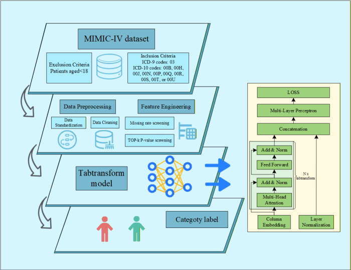
Figure 1. Study workflow and model architecture. This figure illustrates the overall study design, including cohort selection, data preprocessing, feature engineering, dataset splitting, and model development. It also summarizes the TabTransformer architecture used for classification, including feature embedding, Transformer encoder layers, and final classification output. Only the first qualifying admission per patient was included. Please click here to view a larger version of this figure.

Results

Model performance comparison
We compared the proposed TabTransformer model with three baseline models (XGBoost, LSTM with attention, and Temporal Convolutional Networks [TCN]) on the held-out test set. As shown in Figure 2, TabTransformer achieved the highest discriminative performance with an AUC of 0.953 (95% CI: 0.924–0.977), followed by TCN (AUC = 0.937, 95% CI: 0.903–0.967), XGBoost (AUC = 0.857, 95% CI: 0.821–0.890), and LSTM_Attention (AUC = 0.755, 95% CI: 0.707–0...

Discussion

In this study, we developed an attention-based TabTransformer model for in-hospital classification of osteoporosis among adults undergoing spinal neurosurgical procedures and used SHapley Additive exPlanations (SHAP) to explore the main variables driving model output (Figure 5 and Figure 6). The SHAP results suggest that age was the dominant contributor, followed by recurring signals from renal and metabolic markers, hematologic indices, selected medication vari...

Materials

List of materials used in this article

Name	Company	Catalog Number	Comments
Adam optimizer	PyTorch	Included in PyTorch	Used for TabTransformer training
Jupyter Notebook	Project Jupyter	Latest available version	Used for model development and analysis workflow
MIMIC-IV database	PhysioNet	version 3.1; https://physionet.org/content/mimiciv/3.1/	Public de-identified critical care database
Python	Python Software Foundation	Latest available version	Main programming environment
PyTorch	PyTorch Foundation	Latest available version	Deep learning framework used to implement TabTransformer
Relational database management software	Navicat	version 17.0; https://www.navicat.com.cn/	Used for data extraction from MIMIC-IV
scikit-learn	scikit-learn developers	Latest available version	Used for preprocessing, data splitting, and baseline models
SHAP	SHAP developers	Latest available version	Used for model interpretability analysis
SMOTE	imbalanced-learn	Latest available version	Used for minority-class oversampling in the training set
XGBoost	XGBoost developers	Latest available version	Baseline comparison model

References

- Rachner, T. D., Khosla, S., Hofbauer, L. C. Osteoporosis: now and the future. Lancet. 377 (9773), 1276-1287 (2011).
- Khosla, S., Hofbauer, L. C. Osteoporosis treatment: recent developments and ongoing challenges. Lancet Diabetes Endocrinol. 5 (11), 898-907 (2017).
- Jiang, S. D., Dai, L. Y., Jiang, L. S. Osteoporosis after spinal cord injury. Osteoporos Int. 17 (2), 180-192 (2006).
- Kivrak, M., et al. The impact of the SMOTE method on machine learning and ensemble learning performance results in addressing class imbalance in data used for predicting total testosterone deficiency in type 2 diabetes patients. Diagnostics (Basel). 14 (23), 2634 (2024).
- Carvalho, F. R., Gavaia, P. J. Enhancing osteoporosis risk prediction using machine learning: a holistic approach integrating biomarkers and clinical data. Comput Biol Med. 192, 110289 (2025).
- Huang, X., Khetan, A., Cvitkovic, M., Karnin, Z. TabTransformer: tabular data modeling using contextual embeddings. arXiv. , (2020).
- Kapila, A., Takkar, A. Neurological disorders, corticosteroids, and fracture risk: hiding in the hindsight!. J Postgrad Med Educ Res. 56 (2), 61-62 (2022).
- Battaglino, R. A., Lazzari, A. A., Garshick, E., Morse, L. R. Spinal cord injury-induced osteoporosis: pathogenesis and emerging therapies. Curr Osteoporos Rep. 10 (4), 278-285 (2012).
- Landi, F., Liperoti, R., Russo, A., Giovannini, S., et al. Sarcopenia as a risk factor for falls in elderly individuals: results from the ilSIRENTE study. Clin Nutr. 31 (5), 652-658 (2012).
- Romagnani, P., et al. Chronic kidney disease. Nat Rev Dis Primers. 11 (1), 8 (2025).
- Liu, S., Liang, R. Synergistic impact of immuno-nutritional and hypoxia-metabolic disturbances on post-stroke epilepsy: a “two-hit” prediction model and web-based risk calculator. Front Nutr. 13, 1759899 (2026).
- Liu, S., Zhou, J. Trends and development of enhanced recovery after surgery programs in cranial and spinal neurosurgery. Neurochirurgie. 71 (5), 101704 (2025).
- Carvalho, F. R., Gavaia, P. J., Brito Camacho, A. OrthoMortPred: predicting one-year mortality following orthopedic hospitalization. Int J Med Inform. 192, 105657 (2024).
- Liu, S., Liang, R. Risk stratification for intracranial infection after high-grade gliomas surgery: a nomogram development and validation study. Front Oncol. 15, 1697966 (2025).
Access restricted. Please log in or start a trial to view this content.