Single and Two-phase Flow in a Packed Bed Reactor
1. Starting up the apparatus
The apparatus is primarily operated through the distributed control system interface. A Perm P&ID schematic appears and opening/closing automated valves is point and click.
- To establish water flow to either bed #4 or #5, open the inlet and exit valves to the bed being tested and the water supply solenoid.
- Use the flow controller to start water flowing through the bed, raising it gradually. Good starting points are 400 mL/min for bed #4 and 500 mL/min for bed #5. Monitor the differential pressure across the beds. Vary the flow to cover the entire possible range of the DP transmitter.
- Power up the spectrometer equipment and establish communication with the control console. Spectrometer procedures are detailed in the operating manual (SpectraSuite). The calibration of the spectrometer for the fluorescent dye standards will be provided.
- Perform one tracer test each on beds #4 and 5 using 50 ppm dye in DI water as the tracer, at a single average flow rate for each bed.
- Insert the spectrometer probe into the probe sample point (Fig. 1). At the PERM interface, change injection valve status from "Running" to "Charging."
- Inject the tracer using the syringe provided into the sample valve. Change the status to "Running".
- Clean out the injection chamber of the sample valve by changing its status back to "Charging", detaching and loading the syringe with water, then injecting at least 100 mL of water into the valve. When the injected sample has completely exited the bed (spectrometer absorbance returns to base line), change the valve state back to "Running" and let the water flow through the valve for 10 - 15 min at a high flow rate before using it again.
2. Conducting Two-Phase Flow Pressure Drop Experiments
Be sure that the water valves to the beds are closed, the inlet and exit valves to bed #5 are open, the drain valve is open, and that the manual valve for the air to the beds is closed.
- Slowly open the air regulator to establish an air flow (< 5 psig at first). Open the manual valve for the air to the beds.
- Set water flow controller at desired setpoint (700 mL/min) and open manual valve. Route water/air flow to gas-liquid separator (see valving in Fig. 1).
- Confirm that water is exiting to drain. Close the valve to the drain for a period of time to build up a liquid head in the gas-liquid separator. This will result in better separation of the air and water.
- Adjust air flow (typically < 2 SCFM) as desired using the pressure regulator and the dry test meter on the gas exit line. Close the drain valve for short periods of time to get a correct gas flow reading on the wet test meter.
- Conduct two-phase flow pressure drop (use DP transmitter) experiments using bed #5, at multiple air rates. Try to cover the range of the DP transmitter. Disconnect the dry test meter if you see water exiting from the gas exit line.
Source: Kerry M. Dooley and Michael G. Benton, Department of Chemical Engineering, Louisiana State University, Baton Rouge, LA
The goal of this experiment is to determine the magnitude of maldistribution in typical packed bed reactors in both single phase and two-phase (gas-liquid) flow and evaluate the effects of this maldistribution on pressure drop. The concepts of residence time distribution and dispersion are introduced through the use of tracers, and these concepts are related to physical maldistribution.
Channeling in a single-phase flow can occur along walls or by preferential flow through a larger portion of the bed cross-section. Channeling in two-phase flow can result from even more complex causes, and simple two-phase flow theories seldom predict pressure drops in packed beds. A design goal is always to minimize the extent of channeling by finding the optimal bed and particle diameters for the design flow rates and by packing a bed in a way to minimize settling. It is always important to quantify how much maldistribution might occur and to over-design the unit to account for its occurrence.
The permeameter apparatus measures pressure drop, ΔP, and the concentration of tracer (dye) exiting horizontal packed beds of armored glass for either water, air, or two-phase flow (Figures 1 and 2). Water enters through a control valve and can be routed through manual valves to any of five beds (48" long, 3" I.D.) with different size glass bead dumped (random) packings. The pressure drop is measured using a pressure transmitter. The water flow is measured by a differential pressure (DP, orifice) transmitter and the air flow by a dry test meter (similar to a home gas meter). The dye sample is injected upstream by an automated sampling valve. The exit concentration of the dye from a bed is measured using a UV-Vis spectrometer. Residence time distributions are calculated from the tests and compared to the predictions of theories on dispersion in packed beds. Two-phase flow will be studied in bed 5, which contains the largest particles.
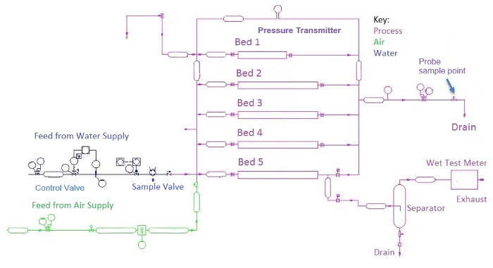
Figure 1: Process and instrumentation diagram of the apparatus.
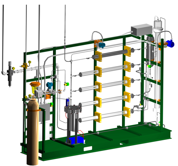
Figure 2. 3-D rendering of the apparatus. Bed #1 is at the top, bed #5 at the bottom. The water control valve is on the left (red bonnet). The DP transmitter is at the top center (blue).
1. Starting up the apparatus
The apparatus is primarily operated through the distributed control system interface. A Perm P&ID schematic appears and opening/closing automated valves is point and click.
- To establish water flow to either bed #4 or #5, open the inlet and exit valves to the bed being tested and the water supply solenoid.
- Use the flow controller to start water flowing through the bed, raising it gradually. Good starting points are 400 mL/min for bed #4 and 500 mL/min for bed #5. Monitor the differential pressure across the beds. Vary the flow to cover the entire possible range of the DP transmitter.
- Power up the spectrometer equipment and establish communication with the control console. Spectrometer procedures are detailed in the operating manual (SpectraSuite). The calibration of the spectrometer for the fluorescent dye standards will be provided.
- Perform one tracer test each on beds #4 and 5 using 50 ppm dye in DI water as the tracer, at a single average flow rate for each bed.
- Insert the spectrometer probe into the probe sample point (Fig. 1). At the PERM interface, change injection valve status from "Running" to "Charging."
- Inject the tracer using the syringe provided into the sample valve. Change the status to "Running".
- Clean out the injection chamber of the sample valve by changing its status back to "Charging", detaching and loading the syringe with water, then injecting at least 100 mL of water into the valve. When the injected sample has completely exited the bed (spectrometer absorbance returns to base line), change the valve state back to "Running" and let the water flow through the valve for 10 - 15 min at a high flow rate before using it again.
2. Conducting Two-Phase Flow Pressure Drop Experiments
Be sure that the water valves to the beds are closed, the inlet and exit valves to bed #5 are open, the drain valve is open, and that the manual valve for the air to the beds is closed.
- Slowly open the air regulator to establish an air flow (< 5 psig at first). Open the manual valve for the air to the beds.
- Set water flow controller at desired setpoint (700 mL/min) and open manual valve. Route water/air flow to gas-liquid separator (see valving in Fig. 1).
- Confirm that water is exiting to drain. Close the valve to the drain for a period of time to build up a liquid head in the gas-liquid separator. This will result in better separation of the air and water.
- Adjust air flow (typically < 2 SCFM) as desired using the pressure regulator and the dry test meter on the gas exit line. Close the drain valve for short periods of time to get a correct gas flow reading on the wet test meter.
- Conduct two-phase flow pressure drop (use DP transmitter) experiments using bed #5, at multiple air rates. Try to cover the range of the DP transmitter. Disconnect the dry test meter if you see water exiting from the gas exit line.
Packed bed reactors are one of the most common types of reactor used in the chemical industry, due to their high conversion rates. Packed bed reactors are typically tubular reactors filled with solid catalyst particles. The reaction occurs on the surface of the solid particle. Thus, small particles enable a high surface to volume ratio and therefore high conversion. Ideally, fluid flows through the reactor in a plug fashion, thus, these reactors are sometimes called plug flow reactors. However, maldistribution of flow or channeling can occur, where flow no longer keeps the even plug-like distribution. This causes the pressure drop in the reactor to decrease and affects the reaction conversion rate. In this video, we will discuss the basics of a packed bed reactor and demonstrate how to measure the pressure drop and flow distribution of one-phase and two-phase flow in the packed bed.
In single-phase packed bed systems, the fluid can be either a gas or liquid. In two-phase reactors, both liquid and gas flow over the solid particles in either co-current or counter-current beds. In both one-phase and two-phase systems, the reactor can be oriented either horizontally or vertically. This solid phase is packed in two ways. Dumped packing is randomly oriented, while structured packing consists of defined geometric networks. The more homogenous the packing, the lower the pressure drop across the bed. An ideal packed bed reactor with single-phase flow can be described by the Ergun equation, which describes the pressure drop across the bed and how it is related to particle size, bed length, void space or porosity, fluid velocity, and viscosity. However, real reactor performance and deviations from ideal must be analyzed experimentally via the tracer method. In the tracer method, a tracer dye, which is assumed to behave similarly to the reactant molecules, is injected into the column. The dye is monitored as it flows through the column, and its concentration upon exit measured as a function of time. In ideal plug flow, the tracer should exit at one instant and the distribution appears as a spike. In a typical column, however, the concentration function takes the form of a Gaussian distribution. This function is then used to calculate the residence time distribution. To quantify the deviation from plug flow, the mean residence time, or the probability that a molecule will exit the column at time T, is calculated as shown. For packed beds, residence time is related to the void volume, which is the product of total bed volume and porosity, divided by the volumetric flow rate, Q. When describing two-phase flow in a packed bed, two simple models are applied. The homogenous model assumes that the gas, liquid, and averaged, or two-phase velocities, are equal. Then the two-phase density is mass velocity, G, divided by the two-phase velocity, UTP. The average two-phase viscosity is defined as shown, where X is the weight fraction of vapor, and mu L and mu G are the viscosities of the respective liquid and gas phases. In the stratified flow model, delta P for each phase is equal to each other. Thus, the Ergun equation for each phase is equal to each other. The pressure drop and both flow rates must be known, while the porosity is computed from the equation. Then the mass balance relates the gas and liquid velocities to the two-phase velocity. Now that you are familiar with the tracer test, let's learn how to carry out the experiment.
Before you start, familiarize yourself with the apparatus, which is operated using a graphical interface. The control system is used to regulate the valves, flows, and various other parameters. Bed number four, which is packed with glass beads and blast sand, is used for the single-phase, while bed number five, packed with glass, is used for the two-phase flow experiment. Start with opening the inlet and exit valve, as well as the water supply solenoid, to bed number four to determine the water flow. Using the flow controller, raise the water flow gradually through the bed and monitor the flow using the differential pressure. Make sure to vary the flow rate to cover the whole range of the DP transmitter. Next, turn on the UV/vis spectrometer and ensure communication with the control console. Using standards of the fluorescent dye, calibrate the spectrometer.
For the test, choose a single average flow rate and a 50 PPM fluorescent dye in deionized water as the tracer. First, insert the spectrometer probe into the probe sample point. Then, using the control system, change the injection valve's status from running to charging. Inject the tracer into the sample valve using the syringe and change the valve status back to running. Monitor the spectrometer absorbance as the tracer passes the bed. To clean the injection chamber for the next experiment, change the status to charging and inject 100 milliliters of water with a clean syringe into the valve. When the absorbance returns to baseline, change the valve to running and purge it with water for 10 to 15 minutes at high flow before the next tracer injection.
Ensure that the water valves to the beds are closed. Check that the inlet and exit valves to bed number five and the drain valve are open. Furthermore, make sure that the manual valve for the air to the beds is closed. Slowly open the air regulator to establish an air flow, Then, open the manual valve for the air to the beds. Next, using the water flow controller, set the flow to 700 milliliters per minute and open the manual valve. Using the valves, route the water and air flow to the gas/liquid separator. Confirm that the water is exiting to drain. To achieve a better separation of air and water, close the valve to the drain temporarily, which will lead to the buildup of a liquid head in the gas/liquid separator. Use the pressure regulator and the dry test meter on the gas exit line to adjust the air flow. Close the drain valve briefly and use the wet test meter to read the gas flow. At a single liquid flow rate, manually vary the air flow at the regulator to cover the range of the DP transmitter and collect the pressure drop data for two-phase flow experiments at bed number five.
Now, let's examine the real flow behavior. For single-phase flow, obtain the residence time distribution. Use the residence time distribution to calculate mean residence time, average porosity, and tracer mass. Compare the calculated tracer mass with the actual value. Next, use the Ergun equation to predict delta P for the water flow experiments. Compare the calculated pressure drops using the calculated porosities to the measured value. For example, in this figure, the minimum porosity for closed pack spheres is 0.36. For bed three and four, the calculated porosity values determined from the residence time distributions are low, leading to the predicted delta Ps being higher than the measured values. This could indicate channeling along the walls of the bed. For the two-phase flows, determine the predicted pressure drop using the homogenous and stratified flow theories and compare it to the measured value. As seen from this table, the pressure drop's calculated using homogenous flow theory, proved to be better than those using stratified flow theory. The high-measured pressure drops suggest severe channeling in the horizontal bed, meaning the liquid was confined to a small portion of the cross-sectional area.
Packed bed reactors are widely used in many areas of industry and research. For example, packed bed reactors are used to convert ground lignocellulosic biomass to hydrocarbon fuel. The first step involves the pyrolysis of biomass to produce bio-oil using a fluidized bed reactor. Like a packed bed reactor, a fluidized bed reactor utilizes solid catalyst particles to facilitate a reaction, but they are suspended in the fluid, rather than packed in a bed. The second step in the process uses a packed bed reactor to convert the bio-oils to fuel. Here, the catalyst particles are ruthenium supported on carbon in the first stage of the reactor, and cobalt molybdenum on alumina in the second stage. The final result is a fuel range hydrocarbon mixture. Packed bed reactors can also be used for enzymatic conversion, such as the digestion of a protein prior to analysis by mass spectrometry. In this example, the reaction takes place on C18 silica particles, packed into a microfluidic reactor. Here, the protein being digested is bound to the particle, while the enzyme flows through the reactor in the fluid. The use of a packed bed reactor for protein digestions, like the example shown here, can improve yield and greatly reduce digestion time and costs.
You've just watched Jove's introduction to single- and two-phase flow in packed beds. You should now understand the basics of a packed bed reactor and how to analyze flow using a tracer test. Thanks for watching!
Obtain the RTDs (E-curves, using Equations 1-2) after subtracting an appropriate baseline (if necessary) from the spectrometer signals. An example of baseline correction for Bed #3 (not used here) is in Figure 3. Using Equations 1-3, calculate the average porosity, tracer mass, mean residence time, variance and variance divided by mean squared from the RTDs. Compare calculated tracer mass with injected mass - if they aren't within expected precision, examine ...
In this experiment the real flow behavior of horizontal packed beds, both in single and two-phase flow, was contrasted to the simpler theoretical models for pressure drop and dispersion (flow spreading in the axial direction, deviating from plug flow). The utility of tracer tests in probing for maldistribution ("channeling") in such beds has been demonstrated, and it has even been shown that certain metrics calculated from the tracer tests can give some idea of the cause of the channeling. These calculations usin...
Chapters in this video
0:07
Overview
1:08
Principles of Flow in a Packed Bed
4:14
Reactor Start-up
5:15
Tracer Test
6:09
Two-phase Flow Experiment
7:26
Data Processing and Results
8:50
Applications
10:20
Summary
Videos from this collection: