Architecting Resilience in Global Freight Forwarding with a Causal AI Framework

Summary

This paper presents a causal AI framework using a Bayesian Network to model systemic risks in global freight forwarding. The goal is to empower strategic decision-making by quantifying how fundamental risks impact key performance indicators (cost, time, reliability), thus enabling proactive and precision-guided risk mitigation.

Abstract

The global freight forwarding industry confronts complex and cascading risks. Conventional analytical methods are often inadequate for managing these risks. This paper proposes a protocol to construct and utilize a causal Artificial Intelligence (AI) framework for systemic risk management. The protocol comprises three primary stages. The first stage involves the construction of a hierarchical Bayesian Network (BN). This BN serves as a causal knowledge graph. Its construction synthesizes domain expertise to map the relationships between fundamental risk drivers and core Key Performance Indicators (KPIs): Cost, Time, and Reliability. The second stage is the parameterization of the BN through the definition of conditional probabilities. This step fuses expert judgment with insights from industry reports. The Noisy-MAX model is employed to manage uncertainty in data-scarce environments. In the final stage, the parameterized model is used to perform predictive simulations and diagnostic analyses. Forward inference generates a baseline risk profile. Concurrently, sensitivity analysis identifies high-leverage intervention points. The application of this protocol yields several critical insights: (i) market supply and demand are identified as the central node of systemic risk. (ii) The model generates distinct risk fingerprints for each KPI. Cost exhibits the highest vulnerability to commercial factors. Time is most sensitive to logistical disruptions. Reliability is uniquely exposed to cybersecurity threats. This work contributes an interpretable AI tool. The tool functions as a what-if engine. It enables freight forwarders to shift from reactive crisis management to proactive, precision-guided risk mitigation.

Introduction

The global freight forwarding industry is the invisible backbone of modern commerce, a multi-trillion-dollar ecosystem orchestrating the flow of goods that underpins global manufacturing and e-commerce¹. Its seamless operation is not a mere logistical convenience but a direct determinant of global economic stability². However, this critical infrastructure is now facing a perfect storm of converging pressures. Intense market competition³, tightening sustainability regulations⁴, disruptive technologies⁵, and unprecedented geopolitical volatility⁶ are no longer isolated challenges. Instead, they have fused into a complex web of systemic risk, where a single disruption -- a port strike, a new tariff, a cyber-attack -- can trigger cascading failures across the entire supply chain. This high level of interconnectedness means that managing risks in silos is no longer viable; survival depends on understanding the system as a whole.

This new reality presents a critical challenge that defies both traditional risk analysis and conventional AI. Traditional tools like Fault Tree Analysis (FTA) are too rigid, failing to capture the probabilistic, interdependent nature of modern risks^7,8. Many existing supply chain resilience models, whether analytical or AI-driven, are designed for asset-heavy sectors like manufacturing, focusing on disruptions to physical flows and inventory buffers^6,9. Recent reviews of the field show that these frameworks typically focus on capabilities rooted in supply chain design, organizational collaboration, and flexibility to withstand disruptions⁹. Concurrently, the rise of artificial intelligence has introduced powerful new tools for risk management. As a systematic review by Zamani et al.⁶demonstrates, AI and big data analytics have shown great promise in enhancing resilience, particularly in forecasting disruptions and optimizing responses when sufficient historical data is available¹⁰.

However, a critical gap remains for the unique context of global freight forwarding. While existing models address physical disruptions, they often lack the granularity to capture the non-physical, yet critical, risk drivers -- such as commercial relationships, information integrity, and macroeconomic pressures -- that define the asset-light, service-centric freight forwarding industry^10,11. This gap in the literature leaves industry leaders flying blind, armed with intuition but lacking a quantitative, intelligent compass for navigating a landscape where data is scarce and causal explainability is paramount for strategic decision-making.

This paper addresses this gap by introducing a novel Causal AI framework specifically designed for the freight forwarding ecosystem. We leverage Bayesian Networks (BNs), a form of probabilistic graphical model that excels at the intersection of data, uncertainty, and expert knowledge¹¹. While Bayesian networks are an established methodology, the novelty of this research lies in the novel architectural design of the models, specifically, their hierarchical structuring tailored to the freight forwarding risk landscape, the integration of disparate commercial and operational risks into a cohesive causal graph, and a parameterization strategy adapted to the industry's data-scarce environment. Unlike purely data-driven models, BNs provide a transparent, white-box representation of the system, enabling both predictive (what-if) and diagnostic (why) reasoning. This approach has proven its power in untangling systemic risks in adjacent high-stakes domains like maritime safety^{11,12,13,14,15,16} and energy systems^{7,8,15,16,17,18,19}. Further evidence of their versatility is found in civil engineering, where they model site-specific project risks^20,21, and in aviation, where they analyze causal factors in drone accidents²². These applications provide robust proof-of-concept, yet no such model exists for the unique risk landscape of freight forwarding, which is characterized by its blend of commercial, operational, and strategic pressures.

Our contribution is threefold, establishing a new paradigm for intelligent risk management in logistics:
Causal AI knowledge graph for systemic risk: We construct the first integrated, hierarchical model for this sector, moving beyond simple risk lists or correlational models. It serves as a knowledge graph that visualizes and quantifies the causal pathways from geopolitical shifts to bottom-line performance, offering an unparalleled, holistic view.
From abstract risk to a strategic digital twin: This model translates abstract risks into their direct impact on the three core KPIs: Cost, Time, and Reliability. It functions as a strategic digital twin, allowing decision-makers to simulate the effects of various disruptions and policy choices, thereby stress-testing their resilience before a crisis hits.
Precision-guided strategic intervention: Through sensitivity analysis, this framework moves beyond reactive crisis management. It pinpoints the highest-leverage intervention points within the system, quantitatively answering critical questions like, Is an investment in cybersecurity or in diversifying carrier relationships more effective at improving delivery reliability?

To ensure the robustness of the causal claims, the proposed framework will be validated using established strategies. These include: (1) simulating targeted interventions to check if the model's predictions align with domain knowledge; (2) conducting sensitivity analyses to assess the impact of potentially omitted variables; and (3) using structure-learning algorithms on available subset data as a cross-check for the expert-defined graph structure.

In essence, this research provides a quantitative, AI-powered compass for navigating the industry's turbulent environment. It empowers stakeholders to make data-informed, causally aware decisions, transforming risk from an uncontrollable threat into a manageable strategic variable, thereby securing both resilience and a competitive edge.

Protocol

Causal AI modeling framework
The causal AI framework was built upon the foundation of Bayesian Networks (BNs), a class of white-box probabilistic AI models. Unlike black-box models like deep neural networks, BNs offer a transparent structure that is ideal for domains requiring explainability and causal reasoning¹¹. The core of the framework was a Directed Acyclic Graph (DAG), which functioned as a causal knowledge graph, explicitly mapping the cause-and-effect relationships within the freight forwarding ecosystem.

The strength of these relationships was quantified using Conditional Probability Tables (CPTs). Every node in BN was associated with a CPT. A node's CPT defines the probability of that node being in any particular state. This probability was conditioned on the states of its parent nodes. For instance, consider the Industry Time Performance node from this model. Its CPT defines the probability of the outcome being Delayed or On-Time for every combination of states of its parent nodes: Transportation Risk, Operational & Compliance Risk, and Partner Risk. This capacity for probabilistic modeling of multi-state dependencies offered a distinct advantage compared to deterministic methods.

The structure of a BN enabled efficient probability calculations. It allowed for the computation of the full joint probability distribution over all variables. Let these variables be X = {X₁, ..., X_n}. This distribution was the product of local conditional probabilities. Each term was the probability of a node given its parent nodes. We denoted the parents of the node X_i as Pa(X_i). This relationship was formulated as:

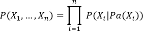
This factorization was the mathematical foundation of BNs. It made inference on complex networks computationally tractable²³.

Crucially for risk management, the framework supports bidirectional probabilistic inference. This allowed for both forward-looking and backward-looking analysis.
Predictive (Forward) inference: This form of inference assesses the potential impact of a specific risk event on overall system performance. For example, it answers the question: If a major cyber-attack occurs, what is the resulting probability distribution for Delivery Time and Cost? This calculation was performed by setting the Cyber Attack node to a specific state as evidence. The BN then propagated this new information through the network.
Diagnostic (Backward) inference: This inference type identifies the most probable causes for an observed outcome. It can answer the question: Given an unexpected surge in costs, what is the most likely root cause? In this scenario, the Cost KPI was set as evidence (e.g., state = High). The network then updated the probabilities of all potential causal factors. This function is essential for effective root cause analysis and focused mitigation efforts²².

Knowledge engineering and causal graph construction
The construction of the causal graph was a critical knowledge engineering phase. Given the scarcity of structured data on systemic risks, we synthesized domain expertise from a targeted review of academic literature and authoritative industry reports, following established methodologies for knowledge-based model construction²⁴. This process transformed qualitative expert knowledge into a formal, machine-readable causal structure, a key advantage of the hybrid AI approach over purely data-driven methods¹¹.

Through this procedure, a comprehensive set of 13 variables was identified and organized into a three-layer hierarchical structure as depicted in Figure 1. It delineated the causal pathways from macro-level drivers to specific performance outcomes. The model constituted a total of 13 variables, or nodes. These nodes are categorized into three distinct layers: (1) Fundamental Risk Drivers (root nodes), (2) Core Industry Risk Areas (intermediate nodes), and (3) Final Industry Performance (leaf nodes). A detailed specification of each variable, its potential states, and its causal parents is presented in Table 1.

Layer 1: Fundamental Risk Drivers
These five exogenous nodes represent the macro-level sources of uncertainty that are largely outside the control of a firm but create the environment in which it operates. This selection is consistent with strategic risk frameworks that analyze the external business environment.
Geopolitics and economy (Node 1): This category combines political and economic risks. The critical role of such macro-environmental factors is a central theme in supply chain risk management. As documented by Wu and Li in their analysis of regulatory impacts like carbon taxes, factors such as trade disputes and volatile regulations directly influence compliance and operational planning⁴. We therefore operationalize these conditions as a root driver with states Unstable and Stable.
Disasters (Node 2): This node represents large-scale disruptions from natural catastrophes and pandemics. The increasing frequency and impact of such events on logistics networks is a central theme in the supply chain resilience literature. These hazard-type risks trigger severe, cascading disruptions throughout the logistics network, underscoring their necessity as a root node in any modern risk framework (https://www.millenniumcargo.com/risk-management-freight-forwarding/).
Market supply and demand (Node 3): This driver is included to capture the intense commercial pressures inherent in the industry. As demonstrated in the equilibrium analysis by Xu et al.³, imbalances between shipping capacity and demand are a fundamental determinant of profitability and partner stability within the shipping service supply chain³. Given its foundational impact on the entire ecosystem, we model it as a primary driver.
Client creditworthiness (Node 4): This node represents a key financial risk originating from the external business environment. The importance of counterparty risk, particularly the financial viability of customers, is a well-established topic in supply chain finance literature, directly impacting cash flow and profitability²⁵. Its inclusion is therefore essential for modeling financial stability.
Cybersecurity environment (Node 5): This node represents the external technological threat landscape. In an increasingly digitized industry, cybersecurity has evolved from technical issues to a systemic operational risk. As highlighted by Garg and Vemaraju⁵, the integration of IoT and AI amplifies this vulnerability⁵, making the external threat environment a critical exogenous factor.

Layer 2: Core industry risk areas
These intermediate nodes represent the direct risks confronting freight forwarders. These risks span operational, business, and technological domains. The nodes function as intermediaries within the causal chain. They translate macro-level drivers into specific, internal challenges.
Transportation risk (Node 6): This node pertains to the physical movement of goods. Its inclusion is fundamental, as transportation is the core function of freight forwarding. It is directly affected by physical disruptions (Disasters) and the reliability of logistics partners (Partner Risk), a recurrent theme in logistics risk management literature (https://genxfreight.co.uk/risk-management-strategies-in-freight-forwarding/).
Operational and compliance risk (Node 7): This category encompasses risks in day-to-day execution and regulatory adherence. The imperative to maintain compliance, particularly concerning sustainability and changing regulations, presents a significant operational challenge that can lead to fines and delays, as analyzed by Wu and Li⁴.
Financial risk (Node 8): This node represents the forwarder's internal financial stability. Its drivers are multifaceted, stemming from macroeconomic volatility (geopolitics and economy), market pressures affecting rates and profitability (market supply and demand)³, and direct counterparty default risk (client creditworthiness)²⁵.
Partner risk (Node 9): Freight forwarders operate within a network of partners (carriers, customs brokers). The reliability of this network is paramount. This node is included to model the risk of partner failures, which can be triggered by large-scale disruptions (Disasters) or severe market pressures that threaten their commercial viability³.
Technology risk (Node 10): This risk pertains to the vulnerabilities of the forwarder's internal digital systems. As firms adopt more advanced technologies like IoT and AI, their internal exposure to IT failures and cyber-attacks increases, making internal technology resilience a distinct and critical risk area⁵.

Layer 3: Final industry performance
These three leaf nodes represent the final business outcomes and correspond to the most widely accepted metrics for evaluating logistics and supply chain performance. They are often referred to as the logistics triangle or golden triangle, where a trade-off often exists between them.
Industry cost performance (Node 11): Representing the total cost of service, this is a primary KPI for any logistics operation. It is the direct outcome of internal efficiencies (operational and compliance risk) and financial stability (financial risk).
Industry time performance (Node 12): Delivery timeliness is a cornerstone of logistics service quality. This KPI is a direct function of the integrity of the physical transit (transportation risk), the smoothness of day-to-day processes (operational and compliance risk), and the reliability of the partners executing the service (partner risk).
Industry reliability (Node 13): Overall service reliability is a broader measure of dependability and trust. This KPI is therefore modeled as being influenced by the integrity of physical transport (transportation risk), operational execution (operational and compliance risk), and the robustness of the technology systems that underpin modern logistics services (technology risk). This hierarchical structure provides a logical organization of the identified risk factors. Furthermore, it enables the Bayesian Network to model the propagation of risk. This propagation flows from external macro-drivers, through specific operational challenges, to the final, measurable business impacts.

Parameterizing the AI model in a data-scarce environment
Model parameterization followed the definition of network structure. This crucial step involved specifying the probability for each node. A comprehensive quantitative dataset for systemic freight forwarding risks is unavailable. Therefore, the probabilities were elicited by a simulated expert panel assessment. This methodology synthesized quantitative insights with qualitative judgments. The inputs were sourced from authoritative industry reports and pertinent academic literature.

Furthermore, risk assessments from literature and expert opinion contain inherent vagueness and subjectivity. Fuzzy set theory was employed to formally account for this uncertainty^19,21. Consequently, the elicited probabilities were conceptualized as fuzzy numbers rather than as single-point values. For presentation clarity, this paper reports crisp probabilities. Each crisp value, however, represents the most representative point (e.g., the centroid) of an underlying fuzzy probability distribution. This approach formally acknowledges that a qualitative statement, such as high risk, corresponds to a spectrum of values rather than a single, precise number.

The parameterization process comprised two primary stages. The first stage defined the marginal probabilities for all root nodes. The second stage defined the conditional probabilities for all child nodes. This second stage utilized the Noisy-MAX model.

Elicitation of probabilities for root nodes
The root nodes of the BN correspond to nodes 1-5. These factors function as the primary sources of risk. The marginal probabilities for these nodes were estimated according to the procedure detailed below. Table 2 presents the final estimated values.
Geopolitics and economy (Node 1): The probability of an Unstable state was estimated at 0.30. This value was derived from reports by institutions such as the World Trade Organization (WTO). These reports document persistent trade tensions and significant global economic volatility (https://www.wto.org/english/res_e/publications_e/publications_e.htm).
Disasters (Node 2): The probability of Frequent disasters was set to 0.15. This estimation was based on analyses from risk intelligence firms. These analyses document the rising frequency of extreme weather events and other large-scale disruptions, including pandemics (https://www.everstream.ai/risk-center/).
Market supply and demand (Node 3): The probability of an Imbalanced market was set to 0.40. This value reflects the well-documented volatility in shipping capacity and freight rates. This volatility is a recurrent theme in major industry reviews (https://unctad.org/topic/transport-and-trade-logistics/review-of-maritime-transport).
Client creditworthiness (Node 4): The probability of Poor creditworthiness was estimated at 0.10. This figure was based on global corporate default studies. Such studies quantify the baseline risk of non-payment in business-to-business transactions (https://www.spglobal.com/ratings/en/regulatory/annual-reviews).
Cybersecurity environment (Node 5): The probability of a Hostile environment was set to 0.25. This estimation was informed by reports on digital threats. These reports document the growing volume and sophistication of cyber-attacks targeting supply chains and critical infrastructure (https://www.pwc.com/gx/en/issues/cybersecurity/digital-trust-insights.html).

Elicitation of conditional probabilities using Noisy-MAX
Defining Conditional Probability Tables (CPTs) for nodes with multiple parents is a complex task. The Noisy-MAX model was therefore employed to manage this complexity²⁶. This model is a generalization of the well-known Noisy-OR framework. This approach is highly suitable for knowledge-based modeling because it significantly simplifies the elicitation process. The model reduces the number of parameters required for each node. Instead of a full CPT, only two parameter types were estimated for each child node:
Independent influence probabilities (ρ_i): This parameter quantifies the probability of a specific causal mechanism. It represents the chance that a single parent factor, acting alone, causes the child node to enter its high-risk state. The estimation of these probabilities is anchored in an analysis of high-impact, well-documented industry case studies. For instance, consider the influence of the Cybersecurity Environment on operational outcomes. The widely cited NotPetya cyberattack on Maersk provides a pertinent example. This event serves as a real-world exemplar of a single technological failure causing global operational paralysis. This case, therefore, offers a defensible basis for estimating a high independent influence probability for this specific causal link (https://www.wired.com/story/notpetya-cyberattack-ukraine-russia-code-crashed-the-world/).
Leak probability (ρ₀): This parameter captures the influence of all unmodeled background causes. These residual factors can also lead the child node to enter its high-risk state. The leak probability thus represents the baseline risk. This risk exists even when all explicitly modeled parent factors are in their favorable, low-risk states.
The elicited parameters for all intermediate and leaf nodes are presented in Table 3. The estimation of these values is derived from a synthesis of authoritative industry reports and well-documented case studies. The following sections provide the specific rationale for each parameter.

Rationale for intermediate node probabilities:
Transportation risk (Node 6): The influence of Disasters is high (0.70). This value accounts for their direct and severe impact on physical infrastructure (https://www.everstream.ai/risk-center/). The influence of Partner Risk is also significant (0.60). Carrier failures lead to immediate transport cessation. The Hanjin Shipping collapse serves as a prominent example of this effect (https://unctad.org/publication/review-maritime-transport-2024). The low leak probability (0.05) represents minor, isolated physical failures.
Operational and compliance risk (Node 7): The influence of an unstable geopolitical environment is set to 0.50. Such an environment creates significant compliance uncertainty and operational hurdles⁴. The impact of partner risk is also substantial (0.40). Partner non-performance directly causes operational and contractual failures. The leak probability is higher (0.10) to account for the wide spectrum of unmodeled internal factors, such as human or process errors.
Financial risk (Node 8): Several factors strongly influence this risk. First, poor client creditworthiness (0.90) constitutes the most direct threat. It represents the high probability of financial loss from customer default²¹. Second, the imbalanced market supply and demand (0.80) is highly influential. It directly impacts freight rate volatility and profitability³. Third, an unstable geopolitics and economy (0.60) pose a strong financial risk through currency and fuel price fluctuations. The very low leak probability (0.02) implies that significant financial distress is almost exclusively attributable to these major economic drivers.
Partner risk (Node 9): Imbalanced market conditions are the primary driver of this risk (0.70). Intense competition and low freight rates can push carriers towards insolvency. Disasters are also a significant cause (0.50). They can disable regional partners or disrupt their operational capacity. The leak probability is set to a low 0.05. This value represents the baseline risk of partner failure due to idiosyncratic reasons, such as internal mismanagement, which is not captured by major market or disaster events.
Technology risk (Node 10): This risk is directly and strongly influenced by a hostile cybersecurity environment (0.60). This reflects the high probability that increased external threats lead to internal system compromises⁵. The relatively high leak probability (0.10) accounts for internal technological issues independent of external attacks, such as software bugs or hardware failures.

Rationale for leaf node probabilities:
Industry cost performance (Node 11): High financial risk is the primary determinant of a high-cost outcome (0.90). Factors like customer default have an immediate and severe impact on profitability. High operational and compliance risk is also a very strong contributor (0.70). It leads to costs from inefficiencies, fines, and error correction. The extremely low leak probability (0.01) suggests that major cost overruns are almost exclusively caused by these two core risk areas.
Industry time performance (Node 12): High transportation risk is the most direct cause of a delayed shipment (0.85). High partner risk is nearly as influential (0.75), as forwarders depend entirely on partner execution. The influence of operational and compliance risk (0.60) is significant but comparatively lower. Some operational issues, like customs delays, may not jeopardize the entire delivery timeline (https://lpi.worldbank.org/). The very low leak probability (0.02) reflects a key assumption. If transportation, operations, and partners all perform reliably, the probability of a significant unexplained delay is minimal.
Industry reliability (Node 13): The perception of low reliability is most strongly influenced by failures in the core physical service (Transportation risk, 0.80). Technology risk is the second major driver (0.65). System outages or data breaches severely undermine client trust and service integrity. Operational and compliance risk (0.50) is another significant contributor, as consistent operational failures erode the perception of dependability. The leak probability (0.03) accounts for other minor factors affecting client perception.

Computational protocol for model implementation
Model construction: We launched GeNIe and created 13 Chance nodes, naming them as per Table 1. We used the Add Arc tool to draw causal links between the nodes, replicating the structure shown in Figure 1 (Visual checkpoint 1: The final network structure must match Figure 1).
Parameterization: For each node, we opened Properties to define its states (Table 1). For root nodes, we entered the marginal probabilities from Table 2 in the Definition tab. For child nodes, we selected NoisyMAX as the node Type and entered the Independent Causal Influence (ICP) and Leaky parameters from Table 3.
Analysis execution:
Baseline inference: We clicked the Update beliefs icon on the main toolbar to compute the baseline probabilities for all nodes. (Visual checkpoint 2: The results should match the probability values in Figure 2).
Sensitivity analysis: We right-clicked a KPI node (e.g., Cost) to set it as a target, navigated to Network > Sensitivity Analysis, selected the Root Nodes as inputs, and ran the analysis. (Visual checkpoint 3: The generated tornado diagrams should match those in Figure 3).

Results

Baseline intelligence from the causal AI model
We first ran the fully parameterized AI framework to generate a baseline system-wide intelligence snapshot. The model's forward inference calculates the marginal probability distribution for each node, providing a quantitative forecast of the industry's default risk state. The complete profile is illustrated in Figure 2.

Analysis of core industry risks
The model identifies fin...

Discussion

This study proposed and demonstrated a causal AI framework for managing systemic risk in the freight forwarding industry. The findings not only identify critical risk drivers but also highlight the complex, interconnected nature of the risk landscape. This section discusses the broader implications of these findings, the practical applications for various stakeholders, and the limitations of the current research.

The primary contribution of this work lies in the transition from conventional, s...

Materials

List of materials used in this article

Name	Company	Catalog Number	Comments
Causal Model Data	The Authors (via Zenodo)	DOI: 10.5281/zenodo.17255289
GeNIe Academic	BayesFusion	Version 2.3