通过电穿孔法将荧光生物分子导入活体微生物并进行观察

摘要

生物分子研究 体内 对于理解生物体系中分子功能至关重要。本文描述了一种新方法，可实现荧光生物分子（如 DNA 或蛋白质）向活体微生物内部的导入。对 体内 通过荧光显微镜记录的数据也进行了展示和讨论。

摘要

研究生物分子的能力 体内 对于理解分子在生物学背景下的功能至关重要。一种强大的方法是将目标分子与荧光蛋白（如GFP）融合，以研究其表达、定位和功能。然而，GFP及其衍生物的分子尺寸显著大于有机荧光染料，且光稳定性较差，而后者通常被用于 体外 实验，而这可能限制研究的范围。

我们最近介绍了一种基于电穿孔的简单、通用且高通量的方法，可实现带有有机荧光染料标记的生物分子进入活体微生物。本文描述了如何利用电穿孔将标记的DNA片段或蛋白质导入 大肠杆菌 和 Saccharomyces cerevisiæ，如何使用荧光显微镜定量内化分子的数量，以及如何定量电穿孔细胞的存活率。可利用荧光或FRET在单细胞或单分子水平上获取数据。还可实现未标记分子的内化，从而引发可观察的生理反应 体内 最后，讨论了针对特定生物系统优化该方案的策略。

引言

大多数活细胞内的荧光研究依赖于荧光蛋白（如GFP）与目标蛋白的融合表达¹这些荧光标签可用于研究参与基因表达或膜转运等过程的蛋白质的拷贝数、扩散模式或定位情况。^2-7荧光蛋白具有高标记特异性、易于操作，并有大量具有不同光物理和化学特性的变体可供选择¹然而，有机荧光染料仍然是首选 体外 由于其更高的光稳定性（比荧光蛋白稳定多达100倍）^8,9，体积小（体积比荧光蛋白最多小100倍）且易于进行分子内标记（主要通过半胱氨酸残基实现）。上述所有因素对于单分子荧光和FRET研究尤为重要¹⁰.

在过去十年中，已开发出多种内部化方法，这些方法结合了有机标记和体内检测的优势；然而，这些方法要么使用相对较大的多肽标签（例如，TMP、HALO 或 20 kDa SNAP 标签）^11-14，要么需要使用非天然氨基酸¹⁵，或者仅限于大型的单层膜真核细胞（例如，刮取加载、注射器加载、显微注射）^16-19。

本方案描述了一种新颖、简便且高通量的内化方法，该方法结合了有机荧光染料的优势与 体内 观察。为了开发该技术，我们改进了常用于将质粒DNA转染细胞的电穿孔实验步骤^20,21 为了加载微生物，例如 E. coli 或 S. cerevisiæ 使用有机标记的生物分子。该方案包含四个简单步骤：将细胞与标记的生物分子孵育、电穿孔、细胞恢复以及洗涤细胞以去除未内化的生物分子。本文介绍了该电穿孔方案，以及用于研究基于细胞和单分子荧光与FRET信号的细胞成像和数据分析流程。

电穿孔依赖于在低离子强度的细胞悬液中施加高压电场，从而形成瞬时的膜孔，使生物大分子能够进入细胞（图1）^20,21。与质粒DNA转化细菌或酵母类似，细胞在电穿孔前必须经过预处理以确保其具备电转感受态。该过程包括多次用水洗涤的步骤，可提高细胞膜的通透性，并降低细胞悬液的离子强度，以避免电穿孔比色皿中发生电弧现象。在本实验方案中，细胞可按以下方法制备（见实验方案：1.1），也可从商业供应商处购买。

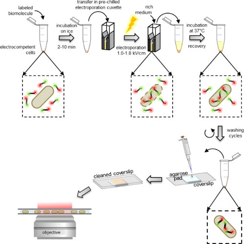
图 1：内化实验流程的示意图。 从左至右：将数微升标记的生物分子加入电转感受态细胞的分装样品中（本示例中为双标记的DNA片段和细菌）；冰上孵育1至10分钟，然后转移至预冷的电穿孔杯中；进行电穿孔，并立即向细胞中加入0.5–1 mL富集培养基；在37 °C（或该生物所需的温度，e.g., 酵母为29 °C）孵育，使细胞恢复；进行5次洗涤步骤以去除未内化的过量标记分子；将最终沉淀重悬于100–200 μl PBS缓冲液中，取10 μl滴加至琼脂糖垫上；用洁净的盖玻片覆盖垫片，并在荧光显微镜下成像（宽场模式或HILO模式）。

在电穿孔前，将电转感受态细胞与标记的生物分子共同孵育，电穿孔操作可使用大多数生物化学实验室中常见的标准电穿孔仪进行。电穿孔后，立即将细胞置于富含营养的培养基中孵育，使其恢复，然后再进行洗涤（图1）。首先通过含有较高盐浓度及一定量去污剂的缓冲液洗涤，去除未被细胞内化的过量标记生物分子（参见实验方案：3.3）。洗涤缓冲液中的盐可破坏未内化标记生物分子与细胞外膜之间形成的非特异性静电相互作用，而去污剂则可破坏非特异性的疏水相互作用。

尽管DNA的内化过程较为直接（图2），但在使用电穿孔法内化标记蛋白时需采取一些预防措施。首先，有机标记蛋白的储存样品中可能仍含有少量游离染料。游离染料分子远小于蛋白质，因此可能优先被细胞内化。为确保观察到的绝大多数内化荧光分子均来自目标蛋白，初始蛋白样品中的游离染料含量应低于约2%（图5）²²。电穿孔后，未内化的标记蛋白也可能非特异性地结合在细胞膜外表面；该现象具有蛋白特异性，每种新蛋白均需单独验证。我们提供了多种方案，可用于去除加载细胞样品中未内化的蛋白（参见实验方案：3.3.3）。

最后，将细胞重悬于少量磷酸盐缓冲液中，并用移液器转移至琼脂糖垫上，以便在荧光显微镜下进行成像。在琼脂糖垫上固定细胞是一种在盖玻片上对细胞进行成像的简单高效方法，且不会破坏细胞的完整性。琼脂糖垫中应含有低荧光背景的培养基。

细胞成像可通过宽场、全内反射荧光（TIRF）或HILO（高倾斜层状光片）显微镜进行。在HILO配置中，激光束进入样品的深度较TIRF更深，但又不像宽场那样照亮整个样品，从而获得更高的信噪比²³。根据所使用的激光功率和时间分辨率，可对内化的生物分子进行计数（通过逐步光漂白分析，图3）、定位或追踪^24-28。使用FRET荧光探针对标记的双标记结构进行内化，可在单细胞或单分子水平上定量FRET（图6）。

根据预期的实验结果和所研究的生物系统，可以调整不同的参数。首先，可通过改变电穿孔前加入细胞的标记生物分子的浓度，来调节每个细胞摄入的物质含量（图2）。电穿孔的电场强度也会影响加载效率和细胞活力；正如预期，随着电场强度的增加，加载效率提高，但电穿孔后细胞的活力下降（图4A）。这两个参数均可通过记录电穿孔后已加载且正在分裂的细胞百分比进行量化。将该活力检测与荧光成像相结合，还可验证生物分子在活细胞内的内化情况，并实现对多个细胞世代的持续观察（图4B）。

综上所述，本方案可实现荧光标记的 DNA 和蛋白质分子在 E.coli 或 S. cerevisiæ²⁶ 中的内化。使用有机荧光染料标记的单个分子可在比荧光蛋白（FPs）长一个数量级的时间尺度上，以高时空分辨率进行追踪。最后，该方法适用于宽场、全内反射（TIRF）和共聚焦检测，以及脉冲激发方案（如 ALEX（交替激光激发^28,29））。

方案

1. Cell preparation

1. Preparation of lab-made electrocompetent bacteria
   1. Prepare a 5-10 ml overnight preculture from a single colony of the E.coli strain of interest in a low-fluorescence medium such as M9 or EZ Rich Defined Medium.
   2. In the morning, inoculate a new 400 ml culture with the overnight preculture such that OD_{600 nm} starts at 0.02. Add to the 400 ml low-fluorescence medium 2.5 ml of 1 M MgSO₄ and 2.5 ml of 1 M MgCl₂.
   3. Grow at 37 °C and 250 rpm until OD_{600 nm} reaches 0.4 to 0.6.
   4. Stop the growth by chilling the culture in an ice-water bath for 10-15 min.
      Note: From now on, carry out all steps at 4 °C (on ice).
   5. Centrifuge the culture 15 min at 1000 x g. Discard the supernatant and resuspend the cell pellet in 250 ml chilled and sterile distilled H₂O.
   6. Repeat the centrifugation and resuspension steps twice, decreasing the volume of water to 100 ml and then 50 ml.
   7. Centrifuge the culture 10 min at 1000 x g. Discard the supernatant and resuspend the cell pellet in 25 ml chilled and sterile distilled H₂O + 10% glycerol.
   8. Repeat the centrifugation and resuspension steps three times, decreasing the volume of 10% glycerol solution to 10 ml, 5 ml, and finally to 500 µl.
   9. Aliquot the cells in aliquots of 20 µl each, flash-freeze in liquid nitrogen and store at -80°C. 
2. Commercial electrocompetent bacterial cells
   1. Dilute a commercial cell aliquot 1:1 with sterile chilled distilled water. Make 20 µl aliquots and store at -80 °C.
3. Preparing electrocompetent yeast
   Note: Electrocompetent S. cerevisiæ cells are prepared before each electroporation experiment and cannot be stored at -80°C as for E. coli.
   1. To start, inoculate 50 ml YPD medium with a single colony of the desired strain of interest.
   2. Incubate at 30 °C and 250 rpm until the OD_{600 nm} reaches 0.6 to 0.8.
   3. Centrifuge cells at 1000 x g for 5 min at 4 °C.
   4. Resuspend the pellet in 25 ml chilled and sterile distilled H₂O.
   5. Repeat the washing steps resuspending twice in 25 ml water and resuspending twice in 2 ml of a chilled solution of sorbitol at 1 M.
   6. Resuspend the cells in 250 µl of 1 M sorbitol and split the cells into 50 µl aliquots. 

2. Agarose pad preparation

1. To remove background fluorescent particles, burn a coverslip in a furnace at 500 °C for 1 hour. “Clean burned” coverslips can be stored for weeks at room temperature covered in aluminum foil.
   Note: Other common cleaning methods such as plasma cleaning or piranha solution might be used as long as the background fluorescence of the cleaned slides remains quasi-null.
2. Prepare a low-fluorescence agarose solution by melting in a microwave oven a 2% agarose - distilled water solution (70 °C). Immediately add 500 µl of the clear 2% agarose solution to 500 µl of 2X low fluorescence culture medium and mix gently.
3. Before it cools down and harden, promptly pipette this agarose - medium solution on a microscope coverslip (No 1.5 thickness) in order to form a pad of roughly 2 cm diameters and a few millimeters height. Avoid bubbles and pop them with a pipette tips if needed.
4. Flatten the pad with a second “burned” coverslip (No 1.5 thickness, see Figure 1).
   Note: This upper coverslip helps form a flat homogeneous pad and protect from dust and drying while cells are being prepared. Minimal medium such as M9 or rich medium such as EZ Rich Defined Medium have been tested for their low fluorescence.

3. Electroporation

1. Incubation
   1. Add up to 5 µl of labeled molecules stored in a low-salt buffer (< 50 mM salt) to a single aliquot of competent cells (20 µl bacteria or 50 µl yeast) and incubate 10 min on ice.
      Note: The concentration of fluorescently labeled molecules in the stock solutions and thus the amount of labeled molecules added to the cell prior to electroporation is directly correlated with loading efficiency (Figure 3, and Discussion). As some proteins are less compatible with low salt condition, the salt concentration in the storage buffer might be increased but the volume of labeled molecules added to the cells prior electroporation then needs to be decreased.
   2. Transfer the mixture of cells and labeled biomolecules into a pre-chilled electroporation cuvette (0.1 and 0.2 cm spacing for bacteria and yeast, respectively). Gently tap the cuvette on the bench to remove any potential bubbles from the solution.
   3. Place the cuvette into the electroporator and apply a high-voltage electric pulse to the solution (0.9 to 1.8 kV/cm, see Discussion for more details on choosing voltage). Such a pulse forms transient pores in the cell membranes allowing labeled biomolecules to diffuse into the cells.
   4. Check that the time constant displayed on the electroporator is between 4 to 6 ms. Lower time constants are often due to too high salt concentration and/or the presence of bubbles in the cuvette, and will lead to very low or no loading of the cells. 
2. Recovery
   1. Immediately after electroporation, add 500 μl of rich medium such as SOC, EZ Rich Defined Medium, YPD or any rich medium to the cells.
   2. Incubate the sample at 37 °C for bacteria and 29 °C for yeast for 2 to 10 min. For viability measurements, where the user wants to evaluate the percentage of cells growing and dividing after electroporation, use a longer recovery time (up to 1 hour) as we observe such lag times before the first cell division.     
3. Washing steps
   1. Wash the cells to remove any non-internalized biomolecules by spinning down the cells for 1 min at 3300 x g and 4 °C. Discard the supernatant and resuspend the cells in 500 μl PBS.
      Note: For each sample, prepare a negative control of cells incubated with the same amount of labeled biomolecules but not electroporated and washed exactly the same way as the main sample.
   2. Repeat the previous steps 3 times.
   3. In the case of protein internalization, optimize the washing procedure depending on the properties and behavior of the labeled protein of interest. The following steps are example of possible optimizations:
      1. Perform the first 3 washing cycles using PBS containing 100 mM NaCl and 0.005% Triton X100 to remove non-internalized proteins which might stick to the outer cell membrane^22,26.
         1. Filter the electroporated cells with a 0.22 µm pore diameter filter fitted inside a 1.5 ml microcentrifuge tube by pipetting the electroporated cells into the filter. Spin down for 3 min at 800 x g and 4 °C. Discard the flow-through. Add 500 µl new PBS over the cells and spin them once again as before and repeat these steps once²².
      2. Add a small amount of protease K (10 ng in 500 μl PBS) during the first washing cycle to allow the digestion of any non-internalized protein.
   4. Spin down the cells for 1 minute at 3300 x g and 4 °C. Discard the supernatant and resuspend the cells in 150 μl of PBS.
   5. Spread the loaded cell solution on the agarose pad by removing the upper coverslip and spreading 10 µl of the cell suspension droplet by droplet. Replace an unused clean burned coverslip (No 1.5 thickness, matching the microscope objective specification) on the top of the pad and press very gently on the slide.
   6. Protect the electroporated cells from light by storing the pads in an opaque box while imaging different samples.

4. Microscope data acquisition

Note: Single-cell and single-molecule fluorescence microscopy in living microorganisms can be performed on any appropriate fluorescence microscope (custom-built or commercial).

1. Settings
   1. Widefield or HILO illumination
      1. Image samples with any TIRF/single-molecule microscope.
         Note: As an example, we use in the laboratory a customized inverted microscope with a TIRF set-up. Beams from a 532-nm and a 637-nm diode laser are combined and collimated before focusing onto the back focal plane of the objective. Fluorescence from the sample is collected through the same objective, separated from the excitation light using a long-pass and a notch filter, and split into red and green channels using a dichroic mirror. The two channels are imaged onto separate halves of the chip of an electron-multiplying charge-coupled device (EM-CCD) camera. Videos are recorded using the kinetic mode. White light images are obtained using a white light lamp and a condenser attached to the microscope as an illumination source.
      2. For general single-molecule observation, set the illumination mode of the microscope to TIRF or HILO²³ (see Discussion for more details about TIRF versus HILO imaging). To set an HILO mode on a TIRF microscope, decrease slightly the angle of incidence of the excitation light to shift the focus slightly higher than the coverslip surface (image the cell interior rather than its lower membrane in contact with the coverslip, see 4.5.4).
      3. For cell-level analysis, long single-molecule tracking experiments or step-wise photobleaching analysis, set the illumination mode of the microscope to a widefield mode ensuring the continuous observation of the whole cell volume and therefore of all internalized labeled molecules. 
   2. Typically, use excitation powers around 0.5-3 mW (~50-400 W/cm²).
      Note: Lower laser powers are useful to achieve long-lived fluorescence observation and tracking (over 1 minute) while higher laser powers might be required for higher spatiotemporal resolution or stepwise photobleaching analysis.
   3. Use exposure times ranging from 15 ms for tracking experiments to 100 ms for more general observation and intensity quantification. Note: Other frame rates and modes can be used such as stroboscopic illumination, particularly for studying fast diffusing species ³⁰.
   4. In the TIRF microscope, record the fluorescence channel on an electron-multiplying CCD (EMCCD) camera at a magnification resulting in a pixel length of ~100 nm/pixel. The TIRF setup is describe in greater details in reference²⁶. 
2. Data acquisition
   1. Switch off or block the laser illumination until the start of the experiment. Switch the EMCCD camera gain off to prevent damage to the camera due to overexposure.
   2. Place the agarose pad sandwich upside down on the microscope stage, with the cell-covered side facing downwards, in order to bring the cell close to the objective. Set the focus on the cells in transmitted light microscopy mode²⁸. Record an image of each cell of view under white light imaging in order to locate the cell outlines before switching off the white light.
   3. Protect the sample from lab ambient light.
   4. For HILO excitation mode, adjust the angle of the excitation beam to each maximum signal-to-noise ratio by illuminating only the section of the sample close to the coverslip surface.
      1. To achieve HILO illumination, focus the laser beam into the back focal plane of a 100x NA 1.4 objective²⁸ (higher numerical apertures such as 1.45 or 1.49 are also suitable). By shifting the focusing lens perpendicular to the beam, the focus moves apart from the objective center so that the beam exits the objective with an angle.
      2. Adjust the lens position in order to maximize the signal-to-noise ratio, intracellular fluorescence intensity versus extracellular background signal.
   5. Switch the camera gain and start data acquisition before switching on the laser.
   6. While recording data, acquire a white-light image of each FOV before or after recording the fluorescence data; this helps to identify cell boundaries in the fluorescence channels.
   7. For viability estimation
      1. Use a low-fluorescence rich medium in the agarose pad to allow cells to grow after electroporation.
      2. Equilibrate the microscope to the optimal temperature for the studied microorganism (37 °C for E. coli, 29 °C for S. cerevisiæ) with an objective heater system.
      3. Record both white light and fluorescence images every 30 min, making sure to remain on exactly the same field of view during the entire data recording. A lag of ≈1 hour is typically observed before cells start to divide. 
   8. Counting the number of internalized biomolecules per cell
      1. Set the laser power to high values (2-3 mW) and long exposure time (100 ms).
      2. Set the illumination to widefield mode in order to illuminate the entire cell.
      3. Record movies as described in step 4.2 making sure to record additional frames (50-100 frames) after the completion of the fluorescence photobleaching.

5. Data analysis

1. General analysis
   1. Analyze the recorded images and movies, both in white light and fluorescence excitations, using an imaging software, such as the free software ImageJ.
      1. In ImageJ, open the images or movies recorded on the microscope (TIF format) in File>Open>Your file location.
      2. To qualitatively compare fluorescence intensities on a computer screen, make sure that all the fluorescence images are displayed with the same brightness and contrast settings in Image>Adjust>Brightness/Contrast. Adjust manually or automatically the settings for a selected image, press “Set” button and select the “Propagate to all the other images” option.
      3. Set the type of information to extract :Analyze>Set Measurements, and select (at least) “Area”, “Standard deviation”, “Min & max gray value” and “Mean gray value”.
      4. To compare cell fluorescence intensities, select the area s of interest using the Freehand selection button of ImageJ and extract the cell intensities in Analyze>Measure. The resulting table contains the measurement values and can be saved and/or copied to other software. The “Mean” value corresponds to the average intensity per pixel in the selected area and can be directly compared between cells or between a cell and the background.
      5. In an electroporated cell sample, a cell is considered loaded if its average intensity per pixel is larger than the average intensity per pixel of the negative control plus 3 times its standard deviation (Av(I _{loaded cell}) > Av(I_–EP)+3*StdDev(I_–EP)). 
   2. Build false-colored fluorescence overlay images and movies in order to evaluate the quality and loading of the samples.
      1. In ImageJ, overlay images such as the white light image and the fluorescence image corresponding to the same FOV in Image>Colors>Merge channels. Select a color for each image (C4(gray) for the white light, C1(red) for red channel, C2(green for green channel…etc.).
      2. Check on the overlay image that the fluorescence is located within the cell boundaries (white light image) and that background fluorescence is low and homogeneous (no bright spots outside the cell boundaries).
      3. Before analyzing a large number of cells, check qualitatively the images corresponding to the negative sample are similar to the empty cell images and display much lower intensities than the electroporated cells.
   3. For viability experiments, count manually the percentages of dividing, non-dividing but visibly intact (identical) and damaged (dead) cells from the same field of view growing over time (See 4.2.6).
   4. Evaluate the viability of at least 200 cells per sample (electroporated, negative control and empty cells) in order to gather enough statistics.
2. Cell-based analysis
   1. Counting the number of internalized biomolecules per cell by step-wise photobleaching analysis
      1. Segment cells by selecting the area of interest using the Freehand selection button of ImageJ and draw a shape surrounding precisely the cell (equivalent to cell membrane).
      2. Extract the cell intensities over time in Image>Stacks>Plot Z-axis Profile. The resulting graph represents the average intensity per pixel for the area within the cell boundary versus each movie frame resulting in a photobleaching curve for that specific cell. It contains an initial exponential decrease of the cell intensity reaching a lower asymptote (background fluorescence). The measurement values and can be saved and/or copied to other software by clicking on “Save” or “Copy”.
      3. Copy and paste the bleaching values into a spreadsheet column (I_raw).
      4. Calculate the average autofluorescence per pixel remaining after photobleaching (I_auto) by averaging the I_raw values obtained for the last 50-100 frames (lower asymptote).
      5. Subtract the average autofluorescence per pixel remaining after photobleaching for that cell from the initial photobleaching curve: I_bleaching = I_{raw -} I_auto.
      6. Use baseline-subtracted photobleaching timetraces (I_bleaching versus frame) showing less than 10 quantized steps to evaluate the average step size (unitary fluorophore intensity) due to the bleaching of a single fluorophore²⁶.
      7. Evaluate the number of internalized molecules per cell by dividing the initial baseline-subtracted cell intensity (I_bleaching at t = 0) by the unitary fluorophore intensity. 
   2. Single-cell FRET efficiencies
      1. Measure the average cells intensity per pixel in both the donor and acceptor emission channels (upon donor excitation) and within the cell boundary for each channel as explain in 5.1.1.4.
      2. Measure the average pixel intensity for the background in each channel from a blank area of the slide.
      3. Subtract this background intensity from the average intensity per pixel. Use these background-subtracted fluorescence intensities to calculate FRET for each cell by calculating the background-subtracted acceptor intensity divided by total (acceptor + donor) background-subtracted intensity upon donor excitation: I_acceptor / (I_acceptor + I_donor) 
3. Single-molecule analysis
   1. Single-molecule tracking and diffusion analysis
      Note: The protocol for tracking diffusing fluorescent molecules in living cells and to evaluate their apparent diffusion coefficient has been described^26,28.
      1. Briefly, fit the images of single fluorophores in each frame by a 2D elliptical Gaussian. Link localized molecules to a track if they appeared in consecutive frames within a window of 5-7 pixels (0.48-0.67 μm). Use a memory parameter of 1 frame to account for the transient disappearance of a fluorophore due to blinking or missed localization.
   2. In vivo smFRET analysis
      1. Manually identify localized molecules inside cells from movies by going through a movie in ImageJ and identify immobile (or fairly immobile) molecules in the FRET (acceptor) channel.
      2. To extract the intensities in the acceptor and donor channel corresponding to an immobile molecule, select the area around the molecule in each channel using the “Oval” selection button of ImageJ (circle around each single fluorophore, using a ∼3-pixel radius) and extract the molecule intensities in Analyze>Measure. The resulting table contains the measurement values and can be saved and/or copied to other software.
      3. Calculate background values per channel from the average pixel intensity from a circle of the same size in a blank area of the slide over all frames analyzed.
      4. Use background-subtracted fluorescence values in the donor and acceptor channels (upon donor excitation) for the fluorescence and FRET time traces, as in the single-cell FRET case (see 5.2.1.7).
         Note: Automated and robust analysis and algorithms have been described in References^26-28,31. 

结果

样品制备

本方案的各个步骤以示意图形式展示于图1中。以细菌摄取双标记（供体和受体染料）DNA片段为例进行说明。DNA内化作用的代表性结果见图2。对于每个电穿孔样品，同时记录了空细胞和未电穿孔细胞的数据（图2）。“空细胞”指既未与荧光生物分子孵育也未进行电穿孔的电感受态细胞；其在荧光通道中的信号强度反映了在相同实验条件下（激光功率、时间分辨率、温度等）的自发荧光水平。“未电穿孔细胞”（也称为–EP，即无电穿孔）作为阴性对照，指已与荧光生物分子孵育但未进行电穿孔的电感受态细胞。这些未电穿孔细胞的荧光水平应与空细胞的自发荧光水平相近，且显著低于已加载并经过电穿孔处理细胞的荧光强度。此结果证实了任何可能黏附于细胞外膜的非内化标记生物分子均已被有效去除。

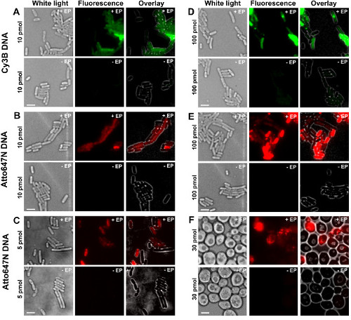
图2：不同浓度下用不同荧光标记的双链DNA在细菌（A-E）和酵母（F）中内化的代表性结果。 从左至右：白光、荧光及叠加图像。-/+ EP 表示在无/有电穿孔条件下孵育。比例尺：3 µm。A. Cy3B标记的双链DNA，10 pmol，E. coli。B. ATTO647N标记的双链DNA，10 pmol，E. coli。C. Alexa647标记的双链DNA，5 pmol，E. coli。D. Cy3B标记的双链DNA，100 pmol，E. coli。E. ATTO647N标记的双链DNA，100 pmol，E. coli。F. ATTO647N标记的双链DNA，30 pmol，酵母。本图经修改自参考文献26。 请点击此处查看此图的放大版本。

每细胞内化生物分子数量的计数

使用光漂白分析法估算每个细胞内化标记生物分子数量的步骤如图3和补充视频2所示，并附有使用不同浓度标记DNA获得的代表性结果。随着孵育的标记DNA初始量增加，细胞摄取效率也随之提高，使用户能够调节每个细胞内的标记分子数量，从“单分子”水平开始<10，补充视频 2B）到“集合”水平（>10，补充视频2A）。估算转染细胞百分比的一种可靠方法是统计电穿孔后细胞荧光强度超过未电穿孔细胞平均荧光强度加3倍其标准差的细胞数量。即，Av(I–EP)+3*标准差(I–EP)，其中 Av 表示平均值，I 表示每个像素的强度，标准差 表示标准偏差，–EP 表示未电穿孔的区域，如图所示 图3.

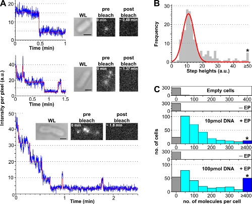
图3：利用光漂白分析技术计数内化分子的数量。 (A) 单细胞光漂白分析。荧光强度时间轨迹示例（蓝色：原始数据；红色：拟合曲线；插图：WL 和荧光图像） E. coli 用ATTO647N标记的dsDNA在漂白前后的负载情况。顶部：单步漂白事件。中部：含有约3个分子的细胞，显示漂白和闪烁现象。底部：含有 >10 个步骤，对应至少 10 个分子。 （B） 来自57个细胞的单步高度强度直方图，这些细胞包含少于6个可区分的台阶，数据通过自动台阶拟合算法获得。单高斯拟合中心位于11 ± 3 a.u.，对应于每秒8100个光子的单体荧光团强度。星号标记的区间汇总了所有大于或等于50 a.u.的台阶高度。 (C) 每细胞内化分子数的直方图，通过将初始荧光强度除以单个荧光分子强度计算得出，细胞经不同浓度ATTO647N标记的dsDNA电穿孔处理。从上到下：空细胞（无处理）即，未与荧光分子孵育且未进行电穿孔）、非电穿孔组（但与荧光分子孵育，记为–EP）以及分别孵育10和100 pmol dsDNA的电穿孔细胞（记为+EP）。空细胞和非电穿孔细胞代表自发荧光背景，而电穿孔细胞显示出内化分子的广泛分布，其中在100 pmol条件下高载量细胞比例更高（≥4个分子，见星号标记的区间）。内化效率（具有内化信号的细胞比例） > 非EP样本的均值 + 3倍标准差）时，10 和 100 pmol 样品的相应值分别为94%和90%。每细胞内化分子的平均数量：10 pmol dsDNA 为 121 ± 106 个分子，100 pmol dsDNA 为 176 ± 187 个分子。成像参数：曝光时间100 ms，宽场照明。比例尺：1 μm。该图已根据参考文献修改 ²⁶. 请点击此处以查看此图的放大版本。

细胞加载与活力检测

除了改变电穿孔前加入细胞的标记生物分子的量外，用户还可以通过选择不同的电场强度来调节分子的内化量（图4，补充视频1）。较高的电场强度可提高内化效率，但会导致细胞活力轻微下降。对于蛋白质内化，使用过滤步骤可能有助于去除未内化的标记蛋白质（见3.3.3.1.1）。在这种情况下，细胞过滤可确保观察到的荧光蛋白确实已进入细菌细胞质内部；然而需要注意的是，过滤也会对细胞活力产生负面影响（更多细节参见参考文献²²）。

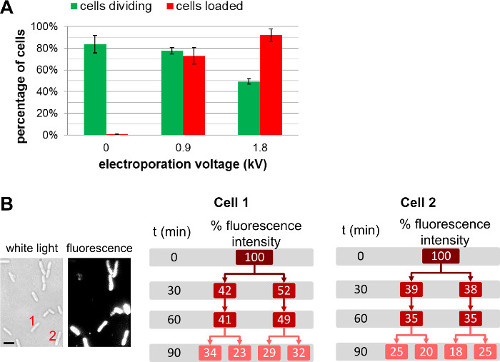
图4：电穿孔电压对细胞加载效率和细胞活力的影响。 (A) 柱状图显示电穿孔场强对加载效率（红色柱）和细胞活力（绿色柱）的影响。在37 °C琼脂糖垫上培养1小时后，未进行电穿孔处理的细胞（0 kV/cm）中有84 ± 8%发生分裂。在相同条件下，经0.9 kV/cm和1.8 kV/cm电穿孔处理的细胞分别有78 ± 3%和49 ± 3%在1小时后分裂。在加载效率方面，在0.9 kV/cm下有73 ± 8%的细胞被成功加载，而在1.8 kV/cm下则有92 ± 6%的细胞被加载。误差线表示三次独立实验的标准差；每次样本及重复实验均分析了超过200个细胞。总体而言，随着电穿孔电压的升高，加载效率提高，但细胞活力略有下降。 (B) 跨越多代的基于细胞的荧光测量结果显示，总体荧光强度在两个子细胞之间均等分配。细胞1和2指代白光图像（左）和t = 0时荧光图像中的细胞编号。比例尺：1 µm。本图改编自参考文献26。

蛋白质内化

蛋白质内化实验的代表性结果如图所示 图5A & B尤其重要的是，在电穿孔之前，应尽可能去除蛋白质样品中残留的游离（未反应）染料。在以下示例中 图5A & B，Cy3b标记的Klenow片段样品（Cy3b-KF，其中KF为Klenow片段） E. coli DNA聚合酶I（66 kDa）仅含有1%的游离染料；该染料对整体细胞载入的贡献可忽略不计。为确保所观察到的荧光分子确实为内化标记蛋白，必须设置两个对照：一是将待测电穿孔样品与未电穿孔但孵育相同量标记蛋白的细胞进行比较，二是与电穿孔相同量游离染料的细胞进行比较。

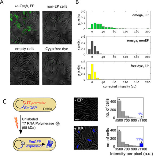
图 5：活细菌中蛋白质的内化。 (A) 荧光叠加视野的代表性图像。细胞在 1.4 kV 电压下进行电穿孔，加入 50 pmol RNAP ω 亚基，该蛋白储存液中仅含 1% 游离 Cy3b 染料。非电穿孔（非–EP）和空细胞的定义如前所述。游离染料的内化浓度与 RNAP ω 电穿孔样本中的浓度相同。宽场模式成像，532-nm 激光激发功率为 1 mW，曝光时间为 50 ms。 (B) (A) 中各样本未经校正的细胞平均荧光强度分布，以总细胞数的比例表示。每样本分割了超过 400 个细胞。本图改编自参考文献 ²²。 (C) 未标记的 T7 RNA 聚合酶（T7 RNAP，98 kDa）进入携带 pRSET-EmGFP 质粒的电感受态 DH5α 细菌的内化情况，该质粒在 T7 启动子控制下编码翡翠绿色荧光蛋白（EmGFP）。左图：实验示意图。中图：荧光叠加图像。右图：非电穿孔样本（上图）和经 T7 RNAP 孵育并电穿孔的细胞（下图）的基于细胞的荧光强度直方图；约 11% 的电穿孔细胞表现出高荧光强度（荧光强度 > 非–EP 样本均值 + 3 倍标准差的细胞比例），表明 EmGFP 的表达。星号表示所有荧光强度大于或等于 1,100 a.u. 的区间。比例尺：3 μm。本图改编自参考文献 ²⁶。

图5C 展示了蛋白质电穿孔的另一项应用。在此实验中，电穿孔导入的蛋白质未标记荧光，但其进入细胞后会触发可观察的荧光信号。该实验用于验证电穿孔蛋白质在细胞质中的存在及其功能活性。未标记的T7 RNA聚合酶（98 kDa）被导入细胞内 E. coli 含有在T7启动子控制下编码荧光蛋白EmGFP的质粒的大肠杆菌DH5α菌株²⁶由于DH5α菌株中缺乏T7 RNA聚合酶基因，本实验中EmGFP的表达需要通过电穿孔将有活性的T7 RNA聚合酶导入细胞图5C)。在使用1 pmol T7 RNAP进行电穿孔后， >11% 的细胞（蓝色柱状图， 图5C）的荧光强度高于阴性对照组（加入等量T7 RNAP但未进行电穿孔）。该结果表明，通过电穿孔进入细胞的部分T7 RNAP分子保持了其完整性 体内 并在细胞质中发挥其预期功能。

体内单分子与单细胞水平的荧光共振能量转移

最后，展示了活体细菌中双标记物种的内化与分析方法 图6 以及补充视频3。由于荧光蛋白融合体并非理想选择 体内 单分子FRET研究中，利用电穿孔将双标记生物分子递送至活细胞的能力是该方法的重要优势之一。 图 6A 展示利用不同FRET DNA标准品（以Cy3B和Atto647N荧光染料作为供体-受体FRET对）负载的细菌的单细胞FRET分析。通过电穿孔将20 pmol三种短的双标记dsDNA FRET标准品（表观FRET效率（E*）分别为0.17、0.48和0.86）导入细胞 体外 （先前已确定）²⁶）。所有DNA均能高效进入细胞（图 6A，左侧）且每个单细胞E*分布的主峰与 体外 结果（图 6A，右侧）。在中、高FRET样本中，观察到部分细胞群体的E*值低于预期，这可能是由于受体漂白和光物理失活、细胞加载量差异（导致信噪比不同）以及DNA降解等多种因素共同作用所致。

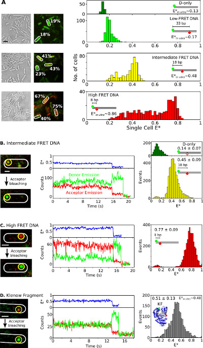
图6：活体细菌中单细胞和单分子FRET观测的代表性结果。 单细菌中的系综与单分子FRET研究 (A) 分析细胞，每种细胞分别加载20 pmol的三种DNA FRET标准品，其FRET效率分别为低（约0.17）、中（约0.48）和高（约0.86）（通过测量获得） 体外 单分子测量（参见参考文献26）。左图：白光与绿色/红色（FRET）荧光叠加图像（比例尺：3 μm）。不同细胞的FRET值示例以白色标出。右图（从上到下）：仅供体（深绿色）、低FRET（浅绿色）、中等FRET（黄色）和高FRET（红色）DNA标准品的未校正细胞水平FRET（E*）直方图。 （B–D） 在体 单分子FRET。细胞分别加载0.25 pmol中等FRET效率的DNA（B图）、0.25 pmol高FRET效率的DNA（C图）和5 pmol双标记的KF（D图）。左列：受体光漂白前后单帧图像的绿色/红色荧光叠加图。中列：对应于黄色圆圈内分子的时间轨迹。FRET效率、供体发射强度和受体发射强度分别以蓝色、绿色和红色显示。右列：每种样品20条时间轨迹中仅含供体分子（绿色）和供体-受体分子（黄色、红色和灰色）的FRET直方图。比例尺：A图为3 μm，B–D图为1 μm。该图改编自参考文献 ²⁶. 请点击此处以查看此图的放大版本。

为了在体内（in vivo）观察 DNA 或蛋白质样品的单分子 FRET（smFRET），可通过电穿孔将少量（0.25 pmol）中等和高 FRET 效率的 DNA 标准品（图6B、C）或 5 pmol 双标记的 KF（以 Alexa647/Cy3B 荧光染料作为 FRET 配对，图6D）导入 E. coli。该浓度可使大量细胞中仅含有少量（n = 1–10）标记分子，从而实现对单个分子的直接定位、追踪和 FRET 监测。部分分子自由扩散，而另一些则表现为固定不动或缓慢扩散（见补充视频3）。双标记生物分子在固定状态下的时间轨迹（图6，中图）持续时间为 1 至 30 秒，呈现出 smFRET 的典型特征：在受体漂白时，供体与受体荧光信号呈反相关变化（例如，t~16 秒；图6B，中图），随后发生单步供体漂白（例如，t~19 秒；图6B）。由这些时间轨迹生成的 FRET 分布图（图6，右图）所得平均值与已发表的体外（in vitro）研究结果^26,31,32高度一致。这些结果证明了对细胞内 DNA 和蛋白质进行定量 smFRET 研究的可行性，并表明蛋白质在电穿孔及内化过程中仍能保持其完整性和结构（T7 RNAP 内化实验结果为此提供了支持）。

补充视频 1： 细胞活力。 左侧：白光图像。右侧：荧光图像。动态 GIF 动画展示了载有 10 pmol Atto647 标记 DNA 的细菌在电穿孔（1.8 kV/cm）后发生分裂的过程。荧光信号的整体表观下降是由于细胞分裂过程中标记 DNA 被稀释，以及每次测量时发生的光漂白所导致。

补充视频 2： 基于细胞的光漂白研究。 A. 一个负载大量标记物的细胞的代表性示例（含有 >100 个 Atto647N 标记的 DNA 分子）。左上图，目标细胞的白光图像（红色矩形框内）。右上图，加载了标记物的细胞视频，显示其荧光在数分钟内的衰减过程。下方，目标细胞整体荧光强度随时间衰减的轨迹。有机荧光染料的光漂白寿命可比荧光蛋白（FPs）高出两个数量级（本例中 Atto647N 约为 41 秒）。B. 一个负载少于 10 个标记分子（本例中为 3 个）的细胞的代表性示例。上方，同 A 组。下方，目标细胞整体荧光强度随时间变化的轨迹，显示单步光漂白和/或闪烁现象，对应于单个有机荧光染料分子的行为。这些台阶的平均高度对应单分子的单位荧光强度（本例中约为 12 a.u.），用于估算每个细胞初始内吞的分子数量。视频在持续红光激光激发下采集，激光功率为 300 µW，每帧曝光时间为 100 毫秒。

补充视频 3： In 体内 单分子FRET 顶部：细胞加载了0.25 pmol的高FRET DNA（如 图6C在nTIRF照明下，使用1 mW绿色（532 nm）激光以每帧50 ms的时间间隔持续监测。每帧图像为绿色和红色（FRET）荧光通道的叠加图像。可观察到扩散和静止的红色（完整）及绿色（单个活性标记）DNA分子。底部：对应于黄色圆圈内分子的时间轨迹。FRET效率、供体发射强度和受体发射强度分别以蓝色、绿色和红色显示。受体漂白事件（红→绿转变）呈反相关，是单分子FRET的典型特征。

讨论

在进行细胞电穿孔和数据采集时，可根据感兴趣的生物系统及实验的具体性质（细胞水平或单分子分析）调整多种参数。例如，在将DNA电穿孔导入细菌时，使用0.25至5 pmol的标记双链DNA片段可导致较低的内化效率，从而实现直接的单分子检测即，无需预先进行光漂白）。当dsDNA用量超过5 pmol时，细胞通常会过度负载，此种情况更适用于单细胞分析。所有标记的DNA在使用前均应通过凝胶纯化，以从DNA储备液中彻底去除游离染料（未反应的荧光染料）。此外，对于单分子FRET实验中可能出现的DNA降解问题，可通过使用含有非天然核酸或具有保护性结构（如发夹环）的DNA来解决，这些结构可保护外切酶可接近的末端。

电穿孔中的另一个可调参数是电穿孔过程中施加的电场强度。较低的电场强度（约 1 kV/cm）会导致较低的装载效率，适用于单分子研究。较高的电场强度（高达 1.8 kV/cm）可提高装载效率；然而，电场强度与电穿孔后细胞的存活率之间存在负相关关系（见图 4）。作为参考，细菌和酵母电穿孔常用的电场强度约为 1.5 kV/cm。时间常数代表该衰减过程的持续时间，是一个便于监测的参数，因为一旦电穿孔杯中发生任何电弧现象，时间常数会立即下降。在正常设置下，时间常数应大于 4 ms；较低的值将导致装载效率低下，甚至产生未成功装载且受损的细胞。大多数电穿孔仪还提供其他可调参数（如“脉冲截断”或“脉冲波形”），可通过调整这些参数来优化细胞的装载效率和存活率。我们已将该方法应用于细菌和酵母，但通过使用适当的电穿孔仪设置，类似的操作流程也应可用于将标记的生物分子导入哺乳动物细胞，因为哺乳动物细胞膜实际上结构更简单（单层脂双层），且电穿孔技术此前已在这些细胞中成功应用²¹。

在内化标记蛋白时，电穿孔前必须从标记蛋白的储备液中完全去除所有游离染料。由于游离染料分子较小，其进入细胞的效率可能高于目标蛋白，且在数据分析过程中难以区分（即使其扩散速度较快）。作为参考标准，用于电穿孔的有机标记蛋白样品中，残留游离染料的含量应低于2%（可通过SDS-PAGE荧光扫描检测）²²。此步骤尤为重要，因为某些染料分子可能非特异性地吸附在经电穿孔处理的细菌或酵母的外膜上。因此，阴性对照样品的单个细胞荧光强度应明显低于电穿孔组细胞，理想情况下应接近空细胞的自发荧光水平（即未与任何荧光标记生物分子共孵育也未进行电穿孔处理的细胞，图2）。

与双链DNA类似，标记蛋白的内化效率与电穿孔前加入细胞的生物分子量相关。然而，其他参数如分子大小和电荷也会影响内化效率。小分子蛋白表现出较高的内化效率，而较大的蛋白（高达98 kDa）虽可成功内化，但效率较低图5)²⁶蛋白质的等电点、与细胞膜的潜在相互作用以及其他理化参数也会影响电穿孔过程中的细胞载入效率。因此，用户需要针对自身实验体系进行优化，同时需注意，标记蛋白的初始浓度过高（>50 μM）将获得最佳的加载效果。电穿孔还提供了一种新工具，可通过将蛋白质及其他生物分子（无论是否标记）导入细胞来干扰并分析细胞功能。T7 RNA聚合酶实验（图5C) 展示了一个实验示例，在该实验中我们可以引入一种能够改变基因表达的生物分子 体内 使用电穿孔法。

在进行单分子荧光实验时，通常优先选择全内反射（TIR）照明模式，因为它仅激发盖玻片表面附近薄层（约100 nm）内的荧光分子，从而提供最佳的信噪比。然而，对活体微生物内部扩散的标记生物分子进行成像时，可能需要更深的照明深度（例如大肠杆菌（E. coli）中可达0.8 µm）。在保持高信噪比的同时，可通过高度倾斜照明（HILO）模式实现更深的照明。另一方面，宽场成像对于逐步光漂白分析尤为重要，此时研究者通过使用高激光功率对整个负载细胞进行完全光漂白，并将初始细胞荧光强度除以单个分子产生的单位强度（单次光漂白台阶），来估算内化分子的数量（图3）。此外，在长时间分子追踪实验中也需要宽场成像，以便在目标分子的运动轨迹遍布整个细胞体积时仍能准确定位其位置。

在本实验方案中，我们展示了电穿孔技术——一种生物学家和生物化学家常用的将核酸递送入细胞的标准方法——如何成为向多种细胞类型递送荧光生物分子的简便手段。这一新颖的高通量技术为在天然环境中观察标记分子提供了独特工具。此外，电穿孔不仅可递送覆盖宽波长范围的荧光染料标记的生物分子，还可递送经多种化学基团修饰的分子，如非天然核苷酸和氨基酸、金属螯合剂、交联剂以及保护基团。若所研究的生物系统对细胞发育并非必需，可将编码目标蛋白的基因敲除（或敲低），从而确保在分子内化后所观察到的蛋白代表了全部（或绝大部分）细胞内蛋白库。本质上，电穿孔技术能够“移植”体外实验的灵活性 体外 将生物偶联物导入活细胞，从而促进合成生物学、系统生物学和相关领域的研究工作 体内 单分子检测

材料

本文使用的材料清单

姓名	公司	目录编号	评论
ElectroMax DH5-alpha 感受态细胞	Invitrogen	11319-019	或任何其他商业或实验室制备的电转化感受态细菌或酵母。
EZ Rich 定义培养基	Teknova	M2105	低荧光富集培养基
MicroPulser 电穿孔仪	Biorad	165-2100	或任何适用于微生物转化的经典电穿孔装置
认证分子生物学级琼脂糖	Biorad	161-3100	用于制备琼脂糖垫的低荧光琼脂糖
显微镜盖玻片，1.5 号厚度	Menzel	BB024060SC	通过在 500 °C 的炉中加热 1 小时以去除背景颗粒
单分子荧光显微镜	自制		详见参考文献
定位分析软件	自编，可在线获取		可用于定位分析的 MATLAB 和 C++ 软件包。
轨迹追踪软件	可在线获取		由 Blair 和 Dufresne 开发的 MATLAB 实现程序。