一种用于在致密核环境中研究染色质的多标记单分子定位显微镜实验方案

摘要

我们提出了一种三色染色质单分子定位显微镜（SMLM）染色与分析方案，可实现常染色质、异染色质和RNA聚合酶II（RNAP II）的可重复空间定位作图。该方案能够在致密的细胞核环境中实现高效的多色标记，包括与染色质相关的靶标，从而实现可靠的同步检测。

摘要

超分辨率显微技术极大地提升了我们突破衍射极限对生物结构进行研究的能力，使其在研究染色质、核纤层以及核仁等致密排列的核结构时不可或缺。染色质具有多尺度的组织结构——从纳米尺度的核小体到微米尺度的结构域——这要求成像技术必须兼具高分辨率和分子特异性。单分子定位显微技术（SMLM），尤其是随机光学重建显微技术（STORM），能够精确绘制表观遗传标记的分布图，为理解染色质的结构与功能提供关键信息。然而，在细胞核环境中进行多标记成像面临独特挑战，包括抗体可及性降低、非特异性结合增加以及荧光染料不稳定等问题。为解决这些问题，我们提出了一种针对高密度核环境优化的顺序免疫标记方案，可实现信号串扰最小化、信号降解较少的稳健三色SMLM成像。该方法包括优化的缓冲液配方、荧光染料选择以及抗体验证策略，以确保多个靶标间可重复且高保真的标记效果。尤为重要的是，我们将该实验方案与一套计算分析流程相结合，利用某一分子靶标的定位点作为空间锚点（种子点），量化不同靶标之间的距离、局部密度以及多标记共定位亲和性。这使得在纳米尺度上对染色质组分进行精细的空间分析成为可能。本方案为致密亚细胞环境中的多组分成像与定量分析提供了可重复的技术框架，为研究染色质等复杂核结构的研究人员提供了一种强有力的工具。

引言

单分子定位显微镜（SMLM）的出现使得在纳米尺度上对生物结构进行前所未有的探索成为可能^1,2,3,4,5。除了单靶标成像外，多色SMLM技术的拓展进一步推动了该领域的发展，能够同时可视化多种分子种类以及亚衍射极限结构之间的空间和时间关系^{6,7,8,9,10,11}。然而，由于细胞核DNA具有高度密集且呈聚合物状的特性，以及抗体在此环境中通透性受限，将多重SMLM技术应用于广泛分布的组蛋白修饰仍面临挑战^{12,13,14,15,16,17,18}。

染色质呈现出一种多层次、多尺度的结构组织，其尺度范围跨越多个数量级，从纳米级的核小体组装到微米级的细胞核架构。在最大尺度上，染色体占据各自独立的染色体区域，在此区域内，基因组进一步划分为A/B区室和拓扑关联结构域（TADs），后者通过环挤压等机制限制远距离调控相互作用。^19,20,21,22在亚200 nm尺度上，染色质以无序聚合物形式组织，由异质性包装结构域（PDs）构成，而非离散的常染色质和异染色质区块，其中转录活跃区域优先定位于PD边界处^{23,24,25,26,27,28,29}在最小尺度上（5–20 nm），染色质由不规则的核小体组装体和核小体簇构成，凸显了其缺乏统一的高阶折叠模式，并强调了基因组结构具有随尺度变化的涌现特性。^24,26,30随着基于测序的技术方法（如染色质免疫沉淀测序和高通量染色质构象捕获）的迅速发展^{19,30,31,32,33}，已鉴定出染色质中尺度组织结构的多种特征^31,32然而，与成像技术不同，这些方法无法捕捉到只有在解析这些结构后才能观察到的空间几何特征。电子显微镜方法，如染色质电子显微镜（ChromEM）²⁴）以及染色质扫描透射电子显微镜（ChromSTEM）²⁵) 揭示染色质具有异质性，并在50–200 nm的尺度上组织成压缩结构域^25,28,29尽管这些技术能够实现高分辨率的染色质压缩结构域识别，但无法提供SMLM所能实现的分子特异性定位。DNA点累积纳米拓扑成像技术（DNA-PAINT）²²和多重荧光 原位 荧光原位杂交（FISH）¹⁹实现高重数检测；然而，DNA-PAINT 受到寡核苷酸富集的细胞核环境中随机结合事件引起的背景噪声显著影响^12,34，而传统的基于热变性的FISH方法则需要破坏天然的染色质折叠结构。先前的研究已应用超分辨率成像技术在此尺度上探究染色质，发现其具有混合型的包装结构域，与此前的相分离模型相悖。^12,23,34,35该方案源自先前发表的一篇论文，该论文探讨了这些发现的生物学意义³⁴因此，鉴于其高分辨率和多重检测能力，基于免疫染色的dSTORM仍然是在接近天然条件下进行多色染色质成像的最可行策略。

该实验方案并非首个实现对两个以上细胞核靶点进行标记的研究，此前已有研究对单个蛋白质复合物或基因进行了标记^12,36。尽管已成功标记核小体上的组蛋白翻译后修饰，染色质的多色单分子定位显微镜（SMLM）标记、成像与分析仍面临重大挑战。首先，在致密的染色质环境中进行免疫染色时，需优化抗体浓度、孵育顺序和缓冲液组成，以确保充分的渗透与结合，同时避免背景信号过高。其次，必须进行全面的多标记分析，因为常染色质、异染色质以及RNA聚合酶等酶之间的相互作用可能远超简单的二元排斥关系。迄今为止，在染色质dSTORM成像中所实现的最大荧光颜色数仍为两种^18,37,38,39。

本文介绍了一种用于三色染色质单分子定位显微成像（SMLM）的稳健实验方案及分析方法。我们的染色流程优化了抗体孵育时间，并采用改进的成像缓冲液⁴⁰，以支持多标记样本的长时间成像。我们进一步描述了用于双色距离分析和三色联合密度分析的计算流程，从而实现对异染色质、常染色质与转录机制之间关系的定量表征。与早期提示异染色质与常染色质相互分离的双色染色质SMLM研究不同，三色染色质成像揭示基因组被组织为多个压缩结构域，其中常染色质和活跃转录区域定位于组成型异染色质核心的外围³⁴。

本方案为多色染色质单分子定位显微镜（SMLM）实验提供了可重复的框架，并建立了适用于多种功能标记的核靶标的分析策略。通过弥补方法学上的空白，该方案能够系统地探索核小体以上水平的染色质结构域组织，既补充了测序和电子显微镜技术，又保留了天然的细胞核结构。本文是已发表论文的扩展版协议³⁴。

方案

NOTE: The subsequent protocol section will be split into the staining process and acquisition process outlined below. For data analysis tutorials please refer the associated publication³⁴ that details analysis of multi-label for labeled histone modifications.

1. Staining process:

NOTE: Throughout the protocol, there is mention of 35 mm dishes or 8 well chambered plates. These are the vessels our group uses for cell culture, however smaller and more efficient methods are possible. Ensure if alternative materials are used that the recommended concentrations for buffers antibodies are maintained. Due to the sequential nature of this protocol, antibody selection is important for successful labeling. We use standard reasoning to ensure that our host antibodies for our targets are different such that our secondary antibodies can target distinct host species effectively minimizing off target effects. Labeling order is determined based on target location within the nucleus. Since we are targeting chromatin packing domains^25,28,34,35 and understand that this is a diffusion driven process, we always label heterochromatic targets first, followed by euchromatin and lastly by RNAPII to minimize steric exclusion in dense heterochromatic regions. Optimization of buffers was done empirically during development of the protocol. We found that inclusion of goat serum after the first target was helpful for reducing off target effects in subsequent steps.

1. Buffer preparation
   1. Buffer components:
      NOTE: For more information about the components including storage and preparation times please see the Table of materials. We recommend that the user have all solutions ready prior to beginning protocol to avoid experimental errors. Quenching solution should be made last.
   2. Make blocking buffer
   3. Weigh out bovine serum albumin (BSA) such that the final concentration in the buffer volume needed for the experiment is 3% and add to a centrifuge tube. Tilt tube to a 45˚ angle so that BSA crystals are spread out in the tube, then add phosphate buffered saline (PBS). This is done to prevent formation of crystal clumps that will not dissolve.
   4. Leave the tube at room temperature until all crystals are dissolved. Do not shake tube or vortex - this will cause bubble formation which will attract proteins to the surface and prevent BSA from dissolving completely.
   5. Once completely dissolved, add Triton X-100 such that that its final concentration is 0.2% (v/v) given the volume chosen in step 1.3. If crystals are not completely dissolved, pipette up and down several times to mix the solution slowly without forming bubbles.
      NOTE: If making modified buffer, include the 10% goat serum in this process. However modified blocking buffers should be made fresh during use and not stored for long times but ensure final concentrations are the same as stated in Table of materials- 3% BSA, 0.2% Triton X-100.
   6. Make washing buffer:
      Repeat steps for blocking buffer in 1.1.2, but use the concentrations listed in the materials section and here for your convenience (0.2% BSA, 0.1% Triton X-100 in 1X -DPBS, and for modified include 1% goat serum)
   7. Make fixative solution:
      1. Add PBS to a centrifuge tube.
      2. Add appropriate quantity of 16% paraformaldehyde to the centrifuge tube for a final concentration of 4%.
         NOTE: Prepare fresh and ready when taking cells out of the incubator. While the current fixative solution does not normally use glutaraldehyde, it can be included and may be useful due to more robust fixation and longer lasting fixation when compared to paraformaldehyde. The setup for dSTORM do not possess capabilities for fluorescence lifetime signals from glutaraldehyde (GA), however users who have the ability may find this useful to separate from fluorophore labeled structures.
   8. Make quenching solution:
      1. Weigh out sodium borohydride on weighing paper.
      2. Prepare centrifuge tube.
      3. Add Sodium borohydride to tube.
      4. Add PBS to tube.
         NOTE: Solution should have bubbles after adding the PBS.
   9. Make imaging buffer:
      1. Dissolve 1,4-Diazabicyclooctane (DABCO) in deionized RNASE, DNASE free water to make 13 mL DABCO solution with a concentration of 1 M.
      2. Add 12 M HCl (~240 µL) until the DABCO is completely dissolved and the pH reaches 8.0.
      3. Prepare 1 M Sodium Sulfite by dissolving in 10X PBS. DTT does not need any preparation.
      4. For final preparation, use prior stocks to make 65 mM DABCO with 30 mM Sodium Sulfite and 30 mM DTT (1 M Stock) in de-ionized water.
      5. Adjust pH through titration with HCl and NaOH until pH is 8.0. Store covered and sealed with Parafilm at 4˚ C no more than 2 months. Monitor pH throughout use.
2. First label staining process details:
   1. Fixation:
      1. Take live cells from the incubator and remove the cell culture medium from the dish. Discard the cell culture medium in a biohazard waste container.
      2. Add enough PBS to cover the cells (1 mL for a 35 mm dish and 500 µL for a chamber glass slide).
      3. Swirl the dish gently to wash the cells with PBS, then remove the PBS from the dish. Discard the PBS in a biohazard waste container.
      4. Add enough fixative solution to cover the cells (1 mL for a 35 mm dish and 500 µL for a chamber glass slide), then leave the cells to fix for 10 min.
      5. While the cells are being fixed, weigh out sodium borohydride for the quenching solution and add it to a centrifuge tube.
      6. Remove the fixative solution from the dish and discard it in the appropriately labeled liquid chemical waste container.
   2. Quenching
      1. Add enough PBS to the dish to cover the surface (1 mL for a 35 mm dish and 500 µL for a chamber glass slide), then place the dish on a shaker (any standard shaker is fine) for 5 min to wash the cells.
      2. Take the dish off the shaker, remove the PBS, and discard it in the appropriately labeled liquid chemical waste container.
      3. Add enough (250 µL, 8-well dish) quenching solution to the dish to cover the surface (1 mL for a 35 mm dish and 500 µL for a chamber glass slide), then place the dish on a shaker for 7 min to quench autofluorescence in the cells.
      4. While the cells are on the shaker, discard the remaining quenching solution in the centrifuge tube in the appropriately labeled liquid chemical waste container.
      5. Take the dish off the shaker, remove the quenching solution, and discard it in the appropriately labeled liquid chemical waste container.
      6. Add enough (250 µL, 8-well dish) PBS to the dish to cover the surface (1 mL for a 35 mm dish and 500 µL for a chamber glass slide), then place the dish on a shaker for 5 min to wash the cells.
      7. Take the dish off the shaker, remove the PBS, and discard it in the appropriately labeled liquid chemical waste container.
      8. Repeat steps 1.2.2.6 and 1.2.2.7 two more times (for a total of 3 PBS washes).
   3. Blocking
      1. Add enough blocking buffer to the dish to cover the surface (250 µL, 8-well dish, 1 mL for a 35 mm dish and 500 µL for a chamber glass slide).
      2. Place the dish on a shaker for at least 1 h to permeabilize the cell membranes and block binding sites (occupy the unspecified sites, so that they would not interfere with the target ones). (While we have tested various times to determine the minimum successful blocking duration as 20 min, we strongly recommend blocking for at least 1 h or longer up to overnight. Optimization might be needed given target and cell line.)
      3. While the cells are on the shaker, prepare primary antibody staining solution (see recommended concentration on vendor website or refer to table in the materials section).
      4. To determine the total volume of staining solutions to make, add 0.5 mL to the volume needed to cover the cells (ex. for one 35 mm dish, prepare a 1.5 mL solution).
      5. Remove the volume determined in section 1.2.3.1 from the blocking buffer stock and add this volume to a new centrifuge tube to prepare the staining solution.
      6. Add an appropriate volume of primary antibody stock to the blocking buffer to get the correct final concentration. Primary antibody stock volumes for several frequently used antibodies can be found in the materials section.
      7. Take the dish off the shaker, remove the blocking buffer, and discard it in the appropriately labeled liquid chemical waste container.
   4. Primary antibody staining:
      1. Add enough primary antibody staining solution to the dish to cover the surface (1 mL for a 35 mm dish and 500 µL for a chamber glass slide), then place the dish on a shaker for at least 1-2 h up to overnight to label the cellular targets.
      2. Take the dish off the shaker, remove the primary antibody staining solution, and discard it in the appropriately labeled liquid chemical waste container.
      3. Add enough washing buffer to the dish to cover the surface (1 mL for a 35 mm dish and 500 µL for a chamber glass slide), then place the dish on a shaker for 5 min to wash the cells.
      4. Take the dish off the shaker, remove the washing buffer, and discard it in the appropriately labeled liquid chemical waste container.
      5. Repeat steps 1.2.4.3 and 1.2.4.4 two more times (for a total of 3 washing buffer washes).
      6. While the cells are on the shaker during the last wash, prepare secondary antibody staining solution (see recommended concentration on vendor website or refer to previous experiments).
      7. To determine the total volume of staining solutions to make, add 0.5 mL to the volume needed to cover the cells (ex. for one 35 mm dish, prepare a 1.5 mL solution).
      8. Remove the volume determined in section 1.2.4.7 from the blocking buffer and add this volume to a new centrifuge tube to prepare the staining solution.
      9. Add an appropriate volume of secondary antibody stock to the blocking buffer to get the correct final concentration. Secondary antibody stock volumes for several frequently used antibodies can be found in the table of materials.
      10. Wrap the centrifuge tube with the secondary antibody staining solution with aluminum foil until ready to add to the cells in the dish.
   5. Secondary antibody staining:
      1. Add enough secondary antibody staining solution to the dish to cover the surface (1 mL for a 35 mm dish and 500 µL for a chamber glass slide), then place the dish on a shaker for at least 40 min to add fluorophores to the labeled cellular targets.
      2. Make sure the dish is covered in aluminum foil to prevent fluorophore bleaching.
      3. Take the dish off the shaker, remove the secondary antibody staining solution, and discard it in the appropriately labeled liquid chemical waste container.
      4. Add enough PBS to the dish to cover the surface (1 mL for a 35 mm dish and 500 µL for a chamber glass slide), then place the dish on a shaker for 5 min to wash the cells.
      5. Take the dish off the shaker, remove the PBS, and discard it in the appropriately labeled liquid chemical waste container.
      6. Repeat sections 1.2.5.4 and 1.2.5.5 one more time (for a total of 2 PBS washes).
      7. The cells can now be imaged or stored for imaging later. If imaging immediately, follow the steps in Acquisition section. If storing for imaging later, continue following the steps below.
      8. Add enough PBS to the dish to cover the surface (1 mL for a 35 mm dish and 500 µL for a chamber glass slide) before storing.
      9. Wrap the dish with parafilm, then with aluminum foil to prevent both liquid evaporation and fluorophore bleaching.
      10. Store the wrapped dish at 4°C until ready to image.
          ​NOTE: For the labels used in this protocol, dishes can be stored for 2-3 days before image quality is significantly impacted; however, different antibodies may have varying stabilities but with proper storage, are stable for some time after the protocol is complete. Storage of a labeled dish for longer than a week is not recommended as the fixative solution is not concentrated enough for long-term stability.
3. Subsequent label staining process:
   1. Blocking:
      1. Refer to 1.2.3.1 - 1.2.3.2 but use blocking buffer with goat serum. The incubation time for blocking can be as short as 1 h, but we recommend longer times with an upper limit of overnight (18-24 h) for these subsequent labels to reduce off target binding. Please refer to previous experiments.
      2. Meanwhile, prepare primary antibody solutions, instead of blocking buffer, in blocking buffer with goat serum.
   2. Primary antibody staining:
      1. Prepare the modified blocking buffer and washing buffer with goat serum and washing buffer with goat serum as detailed in the buffer preparation section.
      2. Refer to step sections 1.2.3-1.2.4 (Blocking and primary antibody staining) using the modified blocking and washing buffers:
         NOTE: The incubation time for primary antibody can be as short as 1 h, and as long as overnight (8-24 h). Although best labeling performance has been achieved with longer incubation times, especially for multi-label. Data in this protocol has been prepared with overnight incubation steps.
      3. Shortly before the incubation time is done, prepare secondary antibody solutions in the modified blocking buffer 1.1.3.
   3. Secondary antibody staining:
      1. Refer to section 1.2.5 (Secondary antibody staining) but use blocking buffer with goat serum.
         ​NOTE: Please note that the incubation time can be as short as 1 h, but we have tested longer times (2-4 h) with similar performance. For the next labels, please repeat section 1.3.

2. Acquisition process

NOTE: For data acquisition, use Nikon Imaging Software (NIS) elements software compatible with the used microscope. Any software that can control filter, light path and camera settings is fine for this protocol. The following Imaging protocol is adapted for Total Internal Reflectance Fluorescence (TIRF) illumination of the sample; however, the labeling protocol is compatible with multiple forms of imaging. Non-TIRF Imaging is possible with this labeling protocol for STORM and is needed for 3D STORM applications. Please use a standard protocol for alternate imaging methodologies.

1. Subsequent label staining process:
   1. Turn on optical components needed and establish connection with proper software. In most cases, like in NIS, the software will not fully initialize unless the computer can properly communicate with the microscope, camera and stage control.
   2. Open NIS Software (or equivalent).
   3. Set up live view: Turn on live view >toggle Keep auto scale > under camera settings set exposure time to 30 ms.
   4. Set up data path for acquisitions.
   5. Navigate to top panel Acquire> Fast Time Lapse> Path
   6. Select proper file name for first acquisition and set number of frames to 10,000.
      NOTE: These steps are taken to limit the time the sample is exposed to the light source once imaging begins.
   7. Ensure that the critical angle and zero angle of TIRF are pre-set prior to acquisition. Please refer to online sources on tutorials on how to accomplish this. As stated before, if you do not use TIRF illumination, this step can be skipped.
   8. Select proper light path for camera and toggle the Epi Illumination option under Lamps(on NIS or equivalent software) to ensure the mirror is set up for wide field illumination from non-laser standard light source.
2. Sample preparation:
   1. Retrieve samples and add imaging buffer (formulation described in section 1.1 Buffer Preparation) to the sample. (Depending on imaging buffer used, different pre-cautions may need to be taken place. Protect samples from light.)
   2. After adding oil to the objective, place sample on stage with proper holder and toggle Perfect Focus and then subsequently focus on sample.
3. Imaging steps:
   1. Find laser spot and navigate to a spot on the dish/plate with no cells.
   2. Toggle TIRF illumination.
   3. Change filter to match the appropriate filter to pass red (or whichever laser used to acquire data for this specific sample) light.
      NOTE: Use a multi-notch filter as described in the table of materials. Multi-notch filter is not necessary, and users can alternatively do imaging non distinct filter cubes designed for the fluorophores used in their staining.
   4. Turn on the laser at the lowest laser power ~ 1 mW(this is dependent on illumination source but is done so to prevent accidental bleaching) and set mirror angle to critical angle.
   5. If no cells are nearby, increase laser power until the laser spot is clearly seen in the live view.
   6. Use the Region of Interest (ROI) tool, draw, set and save ROI where the laser spot is located.
      NOTE: For multi-label samples, please ensure that the laser spots for all necessary light sources for the sample are aligned. In this protocol we use three lasers and ensure that all spots are aligned. This is essential as co-registration of spatial data requires laser alignment.
   7. Return to Epi illumination and the Bright field filter.
   8. Using the ROI definition tool, navigate to find an appropriate healthy cell (e.g. an appropriate HCT116 cell should have adherent, polygonal or oval shape with clear cell boundary).
   9. Center the ROI on the nucleus and click OK to zoom into ROI position (Perform using bright field illumination as the health of cell cannot be determined directly from wide field fluorescent images of the nucleus.
   10. Return to TIRF illumination using the same method used in 2.3.2.
   11. Select appropriate filter for longest wavelength labeled target (in most cases this is far red i.e. Alexa Fluor 647 labeled target). Usually, longest wavelength selected first to avoid photo-bleaching sample with shorter wavelengths in case labeled targets have secondaries that overlap spectra.
   12. On LOW laser power for each needed laser (in multi-label case this would be 3 lasers) turn on laser and illuminate nucleus to ensure that the sample is properly aligned.
   13. Use TIRF controls to ensure that the sample is illuminated with TIRF.
   14. Select appropriate Z-position for acquisition based on needs. However, this can be adjusted right before acquisition.
   15. Set exposure time based on needs of the fluorophores (use anywhere between 10‬-30 ms).
   16. Click Acquire> Fast Timelapse.
   17. Set frames to ≥10,000 and click Apply to create the file in specified directory.
   18. Turn on laser power to 50% and photo-bleach sample.
   19. The nucleus should initially bleach but shortly after (seconds later) it should begin to blink.
   20. Return to desired critical angle and Z-position by toggling saved positions or manually controlling the mirror angle and Z-position and acquire fast time lapse.
   21. Ensure there is no drift in the stage or co-registration of multi-channel images will not be done correctly. Use fiduciary markers (fluorescent microbeads) or save Z-position at beginning of acquisition to use later for drift correction using position save method for multi-point acquisition in the device.
   22. Change filter (or leave it if using multi-notch with pass band for needed fluorophore) and repeat section 2.3.17-2.3.20 (For subsequent labels, make sure to always start on low laser power, adjust parameters and acquire).
4. Data processing:
   1. Load the raw image stack into FIJI using the Bio-Formats plugin. Generate a minimum-intensity projection by selecting Image> Stacks> Z Project and choosing Min intensity as the projection type. Subtract this minimum projection from the raw image stack using Process > Image Calculator. On the resulting image, perform background subtraction (Process > Subtract Background) with a rolling ball radius of 5 pixels.
   2. Define the region of interest (ROI) for individual cells either manually or with the Nuclei Outline plugin (Plugins > GDSC > Cells > Nuclei Outline).
   3. Perform localization analysis on the preprocessed image stack within the defined ROI using the ThunderSTORM plugin (Plugins > ThunderSTORM > Run analysis). Use appropriate parameters for robust localization (e.g., image filter: B-spline, order = 3, scale = 2; peak intensity threshold = 1.5× std (Wave.F1); sub-pixel localization method: Gaussian, sigma = 2; fit radius = 4; fitting method: maximum likelihood). The resulting coordinates can be used to reconstruct the super-resolution image.
   4. For multi-channel experiments, merge channels to generate a composite chromatin reconstructed dSTORM image (Image > Color > Merge Channels).

结果

代表性三色染色质dSTORM图像

所提出的顺序染色方案已验证适用于多种细胞系，包括BJ成纤维细胞、HCT116、AC16、HeLa、MCF10A等。图1 展示了来自BJ成纤维细胞、HeLa和MCF10A细胞的代表性图像。

使用模拟数据集验证分析流程

三色免疫荧光实验方案的开发需要建立一种专门的计算方法，以应对多靶标核单分子定位显微镜（SMLM）数据的复杂性（图2A、2B）。鉴于在致密的染色质环境中多个靶标彼此邻近共存，我们构建了一种点云分析框架，该框架直接处理定位坐标，而非重构图像。该方法利用了针对点云数据已有的丰富聚类分析工具^40,41,42。我们通过受控的模拟数据集，系统评估了该分析流程区分生物学上有意义的空间模式的能力。生成了四种分布类型以代表不同的染色质组织情景：正态分布代表高度聚集的修饰，均匀分布代表分散模式，环形分布模拟排斥区域，随机分布作为组织对照（图2C）。这些模拟模式被锚定在由实验获得的H3K9me3数据中真实的异染色质簇位置上，从而保留了真实的细胞核空间约束条件。该分析框架采用DBSCAN聚类算法（epsilon = 50 nm，最小点数 = 3），这是SMLM数据聚类分析的多种方法之一^40,41,42。为确保聚类参数的合理性，我们此前已描述了一种专为检测染色质压缩结构域而优化的方法³⁴。请注意，当将此步骤作为分析的初始环节时，用户需根据其靶标结构、环境和功能优化参数选择。此处的簇边界通过凸包计算确定，避免了对结构域几何形状的先验假设。我们的验证结果显示，所有模拟分布模式均能通过其独特的距离直方图谱型被清晰区分（图2D）。当以异染色质中心为参考分析定位点时，每种空间组织类型均呈现出特征性的信号模式。我们使用具有明确空间关系的双标记模拟测试了共定位分析（图2E）。空间分离的标记（正态-环形构型）如预期般产生极低的共密度，表现为平坦的分布曲线（图2E）。而重叠的标记模式（正态-随机构型）则表现出随着与参考点距离增加，共密度逐渐下降的趋势，与理论预测一致。这些验证结果表明，我们的分析框架具备在复杂的多靶标数据集中检测和量化空间耦合关系的能力。有关这些模拟数据集生成方法的更多细节，请参阅完整发表的研究文献³⁴。

染色质结构分析的代表性结果

在生物样本中应用我们已验证的分析方法，可揭示通过本方案实现的特征性空间组织模式。利用经过H3K9me3、H3K27ac和RNA聚合酶II三色染色处理的HeLa细胞，我们展示了该方法所具备的分析能力。由于已有超分辨率研究明确证实，在约200 nm尺度上H3K9me3异染色质具有同心环状染色质结构^23,28,35，因此其是理想的参考系统。分析首先通过基于DBSCAN的方法识别异染色质区域，并根据有效半径对其进行分类：小区域（25–40 nm）、中等区域（40–80 nm）和大区域（80–253 nm）。这种按尺寸分层的方法考虑了DNA压缩区域尺寸已知的异质性，其中平均区域半径约为80 nm²⁵。距离测量采用1.5倍簇半径作为搜索窗口（图2B 顶部），以捕获邻近的常染色质及聚合酶信号（图3A、B）。

代表性结果表明，H3K27ac 和 RNA 聚合酶 II 均一致定位于所有类别异染色质边界的附近区域，这与先前的研究^28,44以及关于转录位置相对于染色质结构域分布的模型^23,35,45,46相一致。定量距离分析显示，这些标记物的平均位置非常接近结构域边缘：在大结构域中，H3K27ac 位于边界内 -1.0 nm 处，RNA 聚合酶 II 位于边界外 8.4 nm 处；而在较小结构域中，两者也表现出类似的边缘富集特征，仅有轻微的位置差异。这些测量结果表明，活跃的染色质元件主要集中于抑制性与许可性结构域之间的界面区域，而非被完全排除在外。联合密度分析展示了该实验流程揭示共标记靶标之间空间耦合关系的能力（图 3C-F）。相对于异染色质结构域的分析显示，联合密度峰值出现在结构域边界稍外侧（r/r₀> 1），表明 H3K27ac 与 RNA 聚合酶 II 在边缘区域具有优先共定位特征（图 3G-I）。这些结果展示了该染色与分析流程如何有助于在高度密集的环境中探究复杂的空间关系。

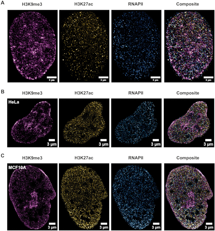
图 1：所用细胞的三色图像。 （A）BJ 成纤维细胞、（B）HeLa 细胞和（C）MCF10A 细胞的三色图像。 请点击此处查看该图的放大版本。

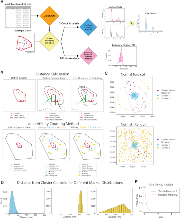
图 2：靶标相对于异染色质簇空间分布的定量分析框架。（A）本研究中用于多通道 SMLM 数据的分析流程。（B）针对已识别异染色质簇的距离至边缘计算示意图及联合亲和计数方法。这两种方法均用于定量确定两个靶标相对于异染色质簇结构的排列方式。（C）在一项研究³⁴中用于确定靶向结构不同生物学组织模式（聚集于结构域内部 vs 围绕结构域 vs 无关联且随机分布）的特定异染色质簇周围的散点分布示例。（D）中心聚集型、随机分布型和环状分布型的距离至边缘直方图，以及（E）模拟情况下的联合亲和曲线。请点击此处查看该图的放大版本。

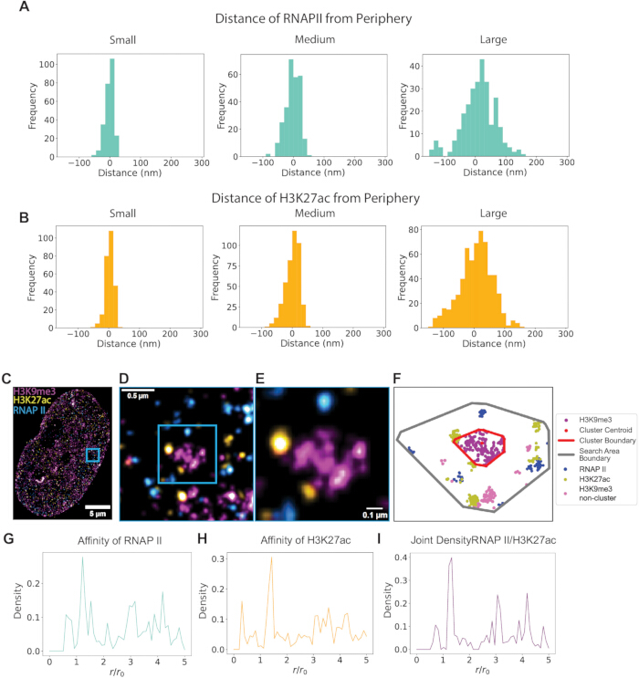
图 3：转录标记物在组蛋白结构域周围的空间定量关系。（A）多标记 HeLa 细胞代表性生物数据中 RNAPII 与（B）H3K27ac 相对于 H3K9me3 簇的小（<40 nm）、中（40–80 nm）和大（>120 nm）结构域的边缘距离直方图结果。（C–E）HeLa 细胞三标 dSTORM 图像示例（H3K9me3、H3K27ac、RNAPII2-S2p），其中包含单个结构域的插图和放大图像。（F）对（E）中所示结构域进行凸包（红色）拟合，分析区域为灰色。（G）在数据集中所有中等大小结构域的分析感兴趣区域（ROI）内，RNAPII 相对于 H3K27ac 的亲和力图，以及（H）H3K27ac 相对于 RNAPII 的亲和力图。（I）所有中等大小结构域在分析 ROI 内 RNAPII 与 H3K27ac 的联合密度图。请点击此处查看该图的放大版本。

讨论

这种三色单分子定位显微技术（SMLM）方案代表了我们在致密细胞核环境中研究染色质组织能力的重要进步。通过结合顺序免疫荧光标记方法与点云空间分析（该分析以定位估计值作为分析的基本点），研究人员得以获得一种强大工具，用于检测不同染色质修饰与活性转录机制之间在纳米尺度上的相互关系，而这些关系此前使用传统显微技术无法被探测到。

该方案的顺序染色策略解决了多靶点细胞核成像中固有的基本挑战。与相对稀疏的细胞质或膜相关结构不同，细胞核染色质靶点密度极高，且空间区域相互重叠。我们改进的封闭方法，在每轮标记后加入针对二抗宿主物种的血清，能有效防止抗体对之间的交叉反应，同时保持靶点特异性。在4°C条件下过夜孵育，可确保抗体充分渗透至整个细胞核体积，这对于实现定量单分子定位显微镜（SMLM）分析所需的均匀标记密度至关重要。该方案可在多种细胞系中稳定获得分辨率达15–20 nm的图像，适用于广泛的染色质结构研究。

以下是成像过程中的故障排除建议。如果细胞核未发生漂白，最可能的原因是样品处的激光强度不足，这可能是由于激光功率设置过低或全内反射角（TIRF）设置不正确所致；此时应通过检查激光光路对准情况、提高激光功率以及仔细调整TIRF角度来进行排查。如果细胞核中闪烁点数量极少但持续保持明亮，表明细胞核漂白程度不足。如果闪烁点非常稀疏且几乎无法观察到细胞核，则最可能的原因是染色失败，应在重复实验前检查所用试剂和抗体。相反，如果细胞核内闪烁点数量非常多（这是理想结果），则需要延长漂白时间，直至能够清晰分辨出彼此分离的单分子闪烁信号。在传统的单分子定位显微镜（SMLM）实验中，通常可借助微管等结构清晰的参考体系来估算合适的标记密度；然而，染色质具有高度异质性的组织结构，并缺乏明确的基准结构，使得此类估算更具挑战性。基于经验优化和先前的研究经验，我们确保有效标记密度达到约每平方微米100个定位点（100 localizations per µm²），以实现对染色质压缩结构域的可靠重建。在本实验方案中，我们未使用任何基准标记物，但若用户具备相关条件，建议使用。在我们的实验中，横向漂移控制在0.2像素以内（小于约5 nm），可忽略不计，因此未使用基准标记物。

选择H3K9me3、H3K27ac和RNA聚合酶II可提供关于染色质在纳米尺度上组织结构的互补信息。H3K9me3可作为理想的空間参考标志，因为它形成离散且界限清晰的簇状结构，代表组成型异染色质，并可通过自动聚类算法可靠地识别。H3K27ac标记与增强子相关的染色质，积极参与基因调控；而RNA聚合酶II则直接指示活跃转录的位点。这三种靶标共同使得研究人员能够探究转录机制和调控性染色质修饰在细胞核结构中相对于异染色质区域的组织方式。

点云分析框架通过实现对致密核环境中的全面空间分析，解决了以往染色质结构研究中的关键局限性。传统的成对比较方法无法捕捉当多种染色质修饰在同一核区域内共存时所产生的复杂空间关系。我们的方法利用联合密度分析，揭示H3K27ac与RNA聚合酶II相对于H3K9me3簇的共定位区域，从而提供从独立的双色实验中无法获得的定量信息。

代表性结果一致表明，染色质呈现出一种紧密关联的组织模式，而非严格的区室化分隔。H3K27ac 和 RNA 聚合酶 II 均优先定位于不同大小异染色质簇的边缘区域，定量测量显示其位置在簇边界 10 nm 范围内，该结果与采用类似方法和转录模型的其他研究团队的发现相一致^{23,28,35,45,46}。联合密度分析表明，活跃的转录机器与增强子相关染色质在异染色质簇周围区域的耦合频率最高。这些发现对简单的相分离模型提出了挑战，并支持一种整合性的组织原则，即不同的染色质修饰在空间上保持紧密邻近，而非形成彼此分离的独立区室。

该方案的模块化设计通过替换靶标，同时保持相同的分析框架，可用来研究多种染色质生物学问题。在复制时序研究中，可将靶标替换为增殖细胞核抗原（PCNA）和微型染色体维持蛋白（MCM）等细胞周期相关蛋白；而在DNA损伤应答研究中，则可靶向γH2AX及修复因子。细胞周期相关研究可检测分裂过程中动态变化的组蛋白修饰，而分化研究则可聚焦于与谱系决定相关的表观遗传标记。这种顺序标记方法适用于任何存在可靠抗体的核蛋白或染色质修饰组合，其主要限制因素为光谱兼容性和交叉反应性。这种灵活性使研究人员能够在维持定量空间分析能力的同时，探究各种细胞过程中染色质动态变化的基本问题。

材料

本文使用的材料清单

姓名	公司	目录编号	评论
Andor iXon Ultra 888电子倍增CCD	安多尔	DU-888U3-CSO-#BV	匿名
牛血清白蛋白	西格玛·奥尔德里奇	A7030	用于挡块和清洗缓冲器。不要在4°下存储基于BSA的阻断缓冲超过1个月;C
长春新工业光电子技术有限公司，型号MGL-FN-532（532纳米）及nbsp;	PSU-H-LED	https://www.cnilaser.com/MGL-FN-532.htm	匿名
相干OBIS激光盒（405 nm， 488 nm， 532 nm， 552 nm， 637 nm）及nbsp;	连贯	1228877	激光与3&ndash同步;10 kW/cm³采样处平均功率，每个波长通道至少收集10,000帧，且不超过bbsp;10–30 MS 获取时间。
DABCO（1,4-地亚氮基环-（2.2.2）-辛烷）	西格玛	D27802	匿名
DBPS（1次）	赛莫飞舍尔	14190-136	匿名
蒸馏水	匿名	匿名	任何蒸馏水都可以;
数字地面电视（二硫代特灵醇），1M	西格玛	43816	匿名
八个井膛盖玻璃	塞尔维斯	C8-1.5H-N	任何玻璃底板都可以，但体积必须根据容器的不同进行调整。
山羊防老鼠 AF568	赛莫飞舍尔	A11004	原料浓度：2 mg/mL 标签后稳定性：2–3天
山羊反兔子 AF647	赛莫飞舍尔	A21245	原料浓度：2 mg/mL 标签后稳定性：4–5天
山羊抗老鼠 A488	赛莫飞舍尔	A11006	原料浓度：2 mg/mL 标签后稳定性：2–3天
H3K27ac一级抗体	赛莫飞舍尔	MA5-23516	库存浓度：1.0 mg/mL
H3K9me3原版抗体	阿布卡姆	AB1769156	库存浓度：1.287 mg/mL
高透明度聚丙烯锥形管 15 mL	康宁	352096	用于定水和淬火溶液
高透明度聚丙烯锥形管 50 mL	科宁	352070	用于40毫升工作中的阻挡和洗涤缓冲液
盐酸（HCl），12M	西格玛	258148	匿名
尼康Eclipse Ti-E，配备完美对焦系统	尼康	TI-DH 611392	倒立显微镜及nbsp;
尼康 SR APO TIRF，100倍放大，1.49 分辨率;	尼康	https://www.microscope.healthcare.nikon.com/products/optics/cfi-apochromat-tirf-series	匿名
普通山羊血清	阿布卡姆	AB7481-1002	在第一个标签完成后使用。应该存在于定型和洗涤缓冲区中
对甲醛 16%	电子显微镜科学	15710	用在固定液中，制作后两周内应用完。保持光线保护，4度;C
磷酸盐缓冲盐水（PBS）10X	安比恩	AM9625	匿名
移液器头 1000 uL	SureOne	02-707-404	任何移液器头都可以，只要它对应体积
RNAPII-PS2	阿布卡姆	AB252855	原汁浓度：0.98 mg/mL
硼氢化钠	赛莫飞舍尔	S678-10	每次淬火缓冲液都用新鲜的。
氢氧化钠（NaOH）	Thermo Fisher等;	A16037.36	匿名
亚硫酸钠	西格玛	S0505	匿名
特里顿 X-100 10%	Thermo Fisher等;	28314	匿名