Live Cell Cycle Analysis of Drosophila Tissues using the Attune Acoustic Focusing Cytometer and Vybrant DyeCycle Violet DNA Stain

Summary

A protocol for cell cycle analysis of live Drosophila tissues using the Attune Acoustic Focusing Cytometer is described. This protocol simultaneously provides information about relative cell size, cell number, DNA content and cell type via lineage tracing or tissue specific expression of fluorescent proteins in vivo.

Abstract

Flow cytometry has been widely used to obtain information about DNA content in a population of cells, to infer relative percentages in different cell cycle phases. This technique has been successfully extended to the mitotic tissues of the model organism Drosophila melanogaster for genetic studies of cell cycle regulation in vivo. When coupled with cell-type specific fluorescent protein expression and genetic manipulations, one can obtain detailed information about effects on cell number, cell size and cell cycle phasing in vivo. However this live-cell method has relied on the use of the cell permeable Hoechst 33342 DNA-intercalating dye, limiting users to flow cytometers equipped with a UV laser. We have modified this protocol to use a newer live-cell DNA dye, Vybrant DyeCycle Violet, compatible with the more common violet 405nm laser. The protocol presented here allows for efficient cell cycle analysis coupled with cell type, relative cell size and cell number information, in a variety of Drosophila tissues. This protocol extends the useful cell cycle analysis technique for live Drosophila tissues to a small benchtop analyzer, the Attune Acoustic Focusing Cytometer, which can be run and maintained on a single-lab scale.

Introduction

Flow cytometry can be used for measurements of cell viability, relative cell size, DNA content and fluorescent protein expression in live cell populations. Due to the replication of nuclear DNA during S-phase, information about DNA content in a population of cells can be used to infer relative percentages in different cell cycle phases ^1-3. This method has become a cornerstone of cell cycle analysis in model systems from yeast to mammals.

The fruit fly Drosophila melanogaster has become an excellent model system for genetic in vivo analyses of cell cycle regulation. The extensive genetic tools available in flies allow for elegant tissue specific and temporally regulated manipulations of cell cycle regulators along with in vivo fluorescent protein-based lineage tracing ^4-6. Flow cytometry has been used to study DNA content in a number of Drosophila cell types, including endoreplicating cells and cultured mitotic cells ^7,8. An important advance for in vivo cell cycle studies was made by de la Cruz and Edgar, with the development of a protocol for flow cytometric analysis of live diploid Drosophila imaginal discs ^9,10, a protocol which has been used and adapted by many labs. This technique, when coupled with genetic in vivo lineage tracing via inducible fluorescent protein expression and tissue specific labeling, allows one to obtain information about gene manipulation effects on overall cell doubling time, cell size and to determine precise timing of cell cycle phases in vivo ^9,11. However this method has thus far relied on the use of the cell permeable Hoechst 33342 DNA-intercalating dye to stain and quantify DNA in live cells, which has limited users to flow cytometers with a UV laser capable of exciting the Hoechst dye. These are generally found only in sorters (i.e. BD FACS Vantage, BD FACSAria) or expensive multicolor benchtop systems (i.e. BD LSR), usually requiring support by institutional flow core facilities.

We have modified the Hoechst-based protocol to use a new live-cell DNA dye from Invitrogen, Vybrant DyeCycle Violet. This dye is compatible with a violet 405 nm laser, more common in smaller benchtop analyzers and available in the small self-contained benchtop analyzer, the Attune Acoustic Focusing Cytometer. Here we present a detailed protocol for cell cycle analysis that can be coupled with cell type, cell size, cell number and lineage analysis in a variety of Drosophila tissues during various stages of development using DyeCycle Violet and the Attune. This protocol expands the number of cytometers suitable for such analysis with Drosophila tissues and provides examples of how this type of live cell cycle analysis can be modified for additional tissue types and developmental stages.

Protocol

1. Fly Husbandry

1. Cross flies of desired genotypes in narrow plastic vials with 10 ml Yeast-Glucose Medium³ or other protein-rich media of your choice. The extensive Drosophila transgenic tools available for tissue specific expression and lineage tracing with in vivo fluorescent protein expression are described in detail elsewhere^4,5. Transfer parents to fresh vials daily to obtain series of 24 hr progeny collections, or for more precise staging, collect embryos on agar plates and transfer newly hatched larva to vials as described¹⁰. To ensure uniform conditions across experiments and avoid overcrowding, the total number of F1 progeny in a single vial should be no more than 100. Depending on the genetic design of the experiment, keep vials in an appropriate incubator until the desired developmental stage.
2. Collect experimental animals: you will need mature larvae at the 3^rd larval instar (L3) at about 110-120 hr of development for larval dissections or white prepupa (WPP) for accurate pupal staging. Dramatic cell cycle changes, including a switch to a non-proliferative state occur at distinct timepoints during metamorphosis^12,13. Therefore correct staging of pupa (within 1 hr of development) is essential for reproducible cell cycle data during metamorphosis. WPP corresponds to 0 hr after pupa formation (0 hr APF) as shown in Figure 1, panel I. Collect WPP in a 35 mm Petri dish on a folded Kimwipe wet with 2.5 ml of water to maintain some humidity. Age pupa until desired stage (hours APF) at appropriate temperature. Note that development proceeds 1.2 times faster at 29 °C and 2.2 times more slowly at 18 °C than at the standard 25 °C¹⁴.
3. Heat-shock animals to activate heat-shock flipase (hs-flp)-induced recombination for lineage-tracing clones if needed^9,11. For the heat-shock of larva, immerse vials in a water bath (set at 37 °C) and ensure larvae are fully submerged. For the heat-shock of pupa, seal the Petri dish with Parafilm and fully submerge it into the water-bath. Be sure to remove Parafilm after the heat-shock, to allow sufficient oxygen exchange for animal survival. Duration of the heat-shock depends on activity of the flipase transgene used and number of clones desired. We routinely use 7-8 min for inducing "flipout" lineage tracing clones¹⁵ in larvae with the hs-flp transgene on the first chromosome and 2-4 min for heat shock of pupae in 35 mm dishes, while the hs-flp transgene on the second chromosome requires a 20 min. heat shock to obtain similar numbers of clones.

The rate of cell division and timing of dissection determines clone size in each tissue. Under normal conditions, we find that clones induced in the larval wing with a 20 min heat shock (using the hs-flp transgene on the second chromosome) and dissected 48 hr later, contain approximately 20-30 well separated clones with sizes ranging from 10 cells per clone to two cells per clone, with an average around four cells per clone. In contrast, a 7 min heat-shock with the same hs-flp transgene of pupae in a Petri dish at 0 hr APF dissected 36 hr later, yields well separated clones (approximately 15-25) ranging from one to four cells with an average of 2.2 cells per clone. Such data can be used to determine the average cell doubling time for the tissue under study.

2. Dissection

1. Gently transfer the larvae/pupae to a clear glass dissection dish containing 1X PBS.
2. Using a dissecting microscope and ample light, gently grasp a larva by the abdomen with a sharp Inox #5 forcep, cut the anterior third with micro-scissors, and invert the anterior third by pushing the mouth area inwards toward the posterior while holding the larval cuticle steady (Figure 1A). Carefully remove opaque fat body and any remaining gut to increase visibility of desired tissues, such as wing, eye or brain. Dissect the desired tissues; cleanly removing wings from trachea and cuticle with forceps, eyes from mouth-hooks, or brain from eyes (Figure 1G).
3. For dissecting pupa; use a forcep to gently grasp a pupa by the anterior tip of the pupal case where there is an air bubble, to avoid damaging the pupa inside (Figure 1C). Forceps or micro-scissors in the opposing hand can be used to help position the floating pupa for proper grasping. Cleanly cut through the posterior tip of the pupa with micro-scissors. This cross-sectional cut should be made at a slight angle toward the dorsal part of the animal, to release the internal pressure without forcing the histolyzed fat into the desired tissues in the thorax and head. Cut carefully along the dorsal median, avoiding the wings and the anterior eye-brain complex. Carefully remove the pupa from the pupal case by grasping the posterior edge of the pupal epidermis and pulling it out of the pupal case (Figure 1D). Poke a small hole in the cuticle anterior to the eye-brain complex with forceps. Using a glass Pasteur pipette with a rubber bulb, gently wash PBS dissection solution through the partially dissected pupa to remove histolyzed fat and any remaining gut tissue. This also effectively lubricates the glass pipette with lipids and proteins, which reduces the incidence of dissected tissues from sticking to the interior of the glass pipette later.
4. To obtain pupal wings, the cuticle enveloping the wing and the wing itself must be pried from the pupa (Figure 1E). This can be done by holding the pupa down by the head with one forcep while using another forcep to either grasp the most posterior tip of the wing cuticle and pulling out or maneuvering the forcep under the wing near the hinge before dislodging it from the side of the carcass (Figure 1E). The wing can then be cut or torn at the hinge to remove it from the body and put in a pile away from the carcasses and other material.
5. To obtain pupal eyes or brain, wash the pupa until the eye-brain complex becomes dislodged and free from the pupa (Figure 1F, 1H). Using a forcep, gently pull the pupal eye away from the brain and save the desired tissue.
6. Do not take longer than 45 min to dissect each sample, as results becomes less accurate the longer cells are left in PBS after opening the animals.

3. Tissue Dissociation and DNA Staining

1. Using a lubricated Pasteur pipette, carefully transfer the dissected tissues into 0.5 ml of Live DNA Stain Solution in a 5 ml polystyrene tube (Figure 1G). Transfer as little PBS as possible (less than 300 μl) into the DNA Stain Solution, as dilution of trypsin will inhibit tissue dissociation.
2. Incubate tubes with shaking at 23 °C at 500 rpm (we use an Eppendorf Thermomixer).
3. Incubate for 70 min, then vortex gently for 5 sec at a medium speed (setting of 5). Excessive vortexing will cause cell disruption and form debris, while under-vortexing will lead to cell clumps. Return the samples to shaking at 23 °C at 500 rpm for an additional 15 to 20 min before vortexing them once more for 5 sec at speed 5.
4. For brains and pupal eyes older than 36hAPF, a modified protocol is required. Dissociate tissues in DNA Stain Solution at 23 °C at 500 rpm for 45-60 min in 1.7 ml microcentrifuge tubes. Then one-by-one manually dissociate large chunks of tissue by transferring to dissecting dish along with about 50 μl DNA Stain Solution and rapid pipetting up and down with a manually drawn Pasteur pipette ¹⁶ (of approximately 100-150 μm opening). Transfer each dissociated specimen with the rest of the 0.5 ml of DNA Stain Solution into a 5 ml tube. Incubate an additional 45-30 min (up to 90 min of total incubation time) at 23 °C with shaking at 500 rpm until clumps are no longer visible.
5. Fully dissociated samples should have very few large visible chunks of tissue, although note that the acellular transparent pupal wing cuticle will not dissociate.

4. Flow Cytometry

1. Turn on the Attune cytometer and open the Attune software. The cytometer lasers should be turned on via the startup menu, and a daily performance test should be performed with Performance Tracking Beads with adequate scores before each day of data acquisition. Fluid levels should be at least half full and waste emptied before the performance test. Details for startup, proper calibration and operation of the Attune can be found in the Attune User Guide ( http://tools.invitrogen.com/content/sfs/manuals/cms_082577.pdf)
2. Design a new template by creating 4 dot plots and 2 histograms in a blank workspace with the parameters indicated in 4.3, or select a previously designed template suitable for the experiment, and indicate the number of samples to be collected. We have provided Attune templates (files in .get format) for live Drosophila cell cycle analysis with Vybrant DyeCycle Violet and GFP or RFP expression in Appendix I.
3. The templates provided include four dot plots and two histograms with the parameters indicated in Figure 2. Channels for detection include: FSC and SSC - forward scatter and side scatter indicating cell size and membrane complexity, VL1 height (H), width (W) and area (A)- indicating Violet laser excitation of DyeCycle Violet staining the DNA, and BL1-A - Blue laser Channel 1 Area, indicating GFP fluorescence. The provided template for RFP analysis is identical to the template for GFP analysis, except that it uses the Blue laser channel 3 (BL3-A), which is optimized for RFP detection.
4. The dot plots in the templates have gates to restrict analysis to the desired populations and to limit debris and cell clumps from analysis (Figure 2). Gate 1 excludes debris and clumps based on SSC vs. FSC (Figure 2A). Gate 2 excludes unstained cells, sub G1 apoptotic cells and cell clumps based upon identification of singlets (VL1Area vs. VL1Width) (Figure 2B). Gate 3 is a derived gate, encompassing cells within gates 1 and 2, and identifies GFP (or RFP) negative cells vs. DNA content based on VL1Height (Figure 2C). Gate 4 is a derived gate, encompassing cells within gates 1 and 2, and identifies GFP (or RFP) positive cells vs. DNA content (Figure 2C). Dot plots of cell size as measured by GFP (or RFP) vs. forward scatter (FSC) are used to generate Gates 5 and 6 (Figure 2D). The two histograms plot DNA content on the X-axis and cell count on the Y-axis for the populations defined by Gate 3 and Gate 4. (Figure 2E and 2F) Histograms can also be included for cell size if desired (not shown). For cell size histograms, populations should be set to Gates 5 and 6, plotting FSC on the X-axis and counts on the y-axis.
5. Set recording to stop at 10,000 GFP or RFP positive events (this will be Gate 4, the derived Gate of Gate 1, Gate 2 and the GFP or RFP positive gate). Ranges from 6,000 - 10,000 GFP positive events have traditionally been the goal for publication quality profiles^9,11. We suggest using a minimum of 15 wings or eyes, that are approximately 50% GFP positive to obtain sufficient Gate 4 events¹⁰ for high quality profiles. However, we have successfully obtained clear data for preliminary cell cycle analysis from as few as 6 wings (Figure 3A). Set the acquisition volume for 300 μl, this will use about 460 μl of the total 0.5 ml sample. Table 2 shows the appropriate threshold and voltage settings provided in the template for the example in Figure 2.
6. Run samples at standard sensitivity or high sensitivity 100 μl/min and record. We find little to no difference in our analysis with the different sensitivity levels. Due to the acoustic focusing of cells, this cytometer can accurately measure samples at very high flow rates. Unlike traditional cytometers, we find no data compromise by acquiring at speeds up to 1,500 events per second. The recorded data files generated by the Attune software are in .fcs format, which is compatible with most cell cycle modeling software.

5. Data Analysis

1. Histograms of cell size and DNA content for GFP (or RFP) positive and negative populations can be compared. They can be manually layered by copying and pasting using Adobe Photoshop software. If the y-axis is set to automatic, the Y-axis will scale with the highest count for each sample. Overlaying two graphs with the Y-axis set to autoscale creates an overlay of histograms with the axes set for the global maximum for each population. This allows easy visual comparison for relative changes in cell cycle phasing, even when total cell numbers of GFP positive and GFP negative populations are not equivalent (example in Figure 3B). Alternatively, a custom y-axis (y-axis manual option) can be set to a fixed value for the histograms. In this case the relative cell numbers for two populations can be compared. As the Attune uses a defined volume of sample per run, absolute quantification of cells for each run, in each gate with percentages of the total population, can be obtained from the statistics table automatically generated during the run in the workspace (example in Figure 3F). Dot plots and histograms can also be easily layered in the Attune software, by simply dragging and dropping different samples from the sample file menu at right onto the desired graph of an open sample for comparison. However to overlay subpopulations from within a single sample (i.e. GFP positive and GFP negative within the same sample), we use Photoshop.
2. Two methods can be used to find relative percentages in different phases of the cell cycle for a population. The approximation method relies upon user defined regions to delineate boundaries of G1, S, G2 and >G2 peaks. This method allows quick and easy estimations of percentages within the user-defined regions (Figure 3E). We set our regions based upon a direct test with Drosophila Kc cells, labeled for S-phase using Ethynyl-deoxyUridine (EdU) incorporation. The second method uses third party modeling software for estimation of cell cycle distribution. We used ModFitLT (Verity Software House) software for example, in Figure 3F.

Results

Figure 2 shows representative results for a larval wing sample, expressing GFP in the posterior half of the tissue, using the provided GFP template. Similar results are obtained with the same tissue type and expression pattern for RFP using the provided RFP template (Figure 3A). The provided templates and voltages (Table 2) are suitable for analysis of larval eyes (Figure 3B), brains and wings, as well as pupal eyes, brains (Figure 3D) and wings. Histograms of relative cell size provided by plotting FSC for populations in Gates 5 and 6 can also be generated (Figure 3C). Gates may need to be adjusted slightly due to differences in cell size for different tissues or differences in fluorescence intensity for different GFP or RFP transgenes. This can be done while running a small test volume of sample (50-100 μl), before hitting record.

Allowing the y-axis (counts) for the cell cycle or cell size histograms to auto-scale (y-axis scale set to automatic) in the Attune software, results in histograms showing the global maximum for each population. Figure 3B-3D shows representative results with GFP positive and GFP negative histograms with y-axis set to the global maximum for each population. Setting a specific y-axis maximum (y-axis scale set to manual with a user defined value), allows for comparison of absolute numbers between populations, which can be useful for comparing proliferation rates, but makes it difficult to compare cell cycle phasing in populations when numbers of GFP positive cells vs. GFP negative cells are vastly different.

Figure 3B shows cell cycle profiles for GFP positive and negative cells in larval eyes, expressing GFP in the posterior using the GMR-Gal4, UAS-GFP transgenes. The overlay reveals the differences in cell cycle phasing of the posterior GFP expressing cells. Figure 3C shows the relative change in cell size between GFP positive and negative cells in B, by plotting cell size as measured by FSC. Figure 3D shows a cell cycle profile from pupal brains at 46h APF. GFP positive cells are lineage tracing clones expressing the G1-S regulators Cyclin D and E2F that disrupt quiescence and lead to S-phase entry, indicated by the red arrow and confirmed by S-phase labeling with incorporation of EdU (Figure 3D inset). This is in contrast to the non-expressing GFP negative cells, which at this stage are normally arrested in G1 (black trace, Figure 3D).

Most cell cycle profiles are used to obtain information about percentages of a population in different cell cycle phases. This can be approximated in the Attune software by creating user defined regions on the histograms delineating G1, S and G2 phases (Figure 3E). The Attune software automatically generates a statistics table for each run, giving the absolute counts of cells within the user defined regions and percentages (Figure 3F). This method works well when comparing relative changes in phase distribution between a control and experimental population. Alternatively, modeling software can be used to estimate percentages in each phase as well as apoptotic cells. We used ModFitLT (Verity Software House) in Figure 3G, which can directly open the .fcs data files generated by the Attune software.

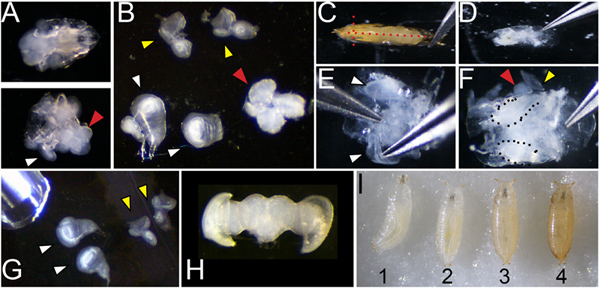
Figure 1. Dissection and staging of larval and pupal tissues. A. Dissection of larvae (of genotype w¹¹¹⁸ shown) at 110 hr of development showing the anterior third before (top) and after (bottom) inversion. White arrowhead indicates a wing attached to the larval cuticle and a red arrowhead indicates the position of the brain B. Wings (white arrowhead; note wing at left is attached to a leg disc, wing at right is torn at the dorsal notum), eyes (yellow) and brain (red) removed from the larvae. C. Dissection of pupa showing positions of cuts with forceps placed at the airspace anterior to the head (red dotted lines) D. Pupa removed from cuticle before washing to remove fat and gut. E. Cleaned pupa showing process of lifting wings for removal F. Cleaned pupa showing wings (dotted) and partially removed eye-brain complex (red and yellow arrowheads). G. Dissected larval wings and eyes showing pipette for transfer. H. Dissected post-mitotic pupal eye-brain complex. I. Correct staging of animals at the larval/prepupa transition; animal 1 is still moving and is too young; animal 2 is at the correct stage to collect, 0hAPF (after pupa formation) it is white and immobile; animal 3 is too old to collect, the darkening of cuticle is evident by 1hAPF; animal 4 is too old to collect already tanned at 2hAPF. Click here to view larger figure.

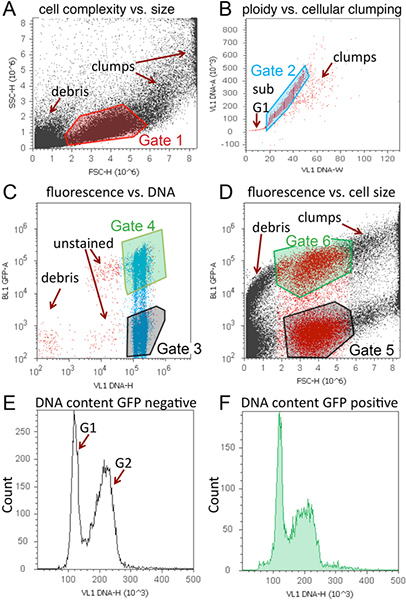
Figure 2. Representative cell cycle analysis of tissues expressing GFP using Vybrant DyeCycle Violet and the Attune. A representative workspace, containing 4 dot plots and 2 histograms is shown for a larval wing sample expressing GFP and Cyclin D in the posterior wing, driven by an engrailed-Gal4 transgene. A. Dot plot of cell size with Gate 1 to exclude debris and clumps. B. Dot plot to discriminate singlets with Gate 2 to exclude unstained cells, sub-G1 DNA content (apoptosis), and clumps. C. Dot plot of GFP vs. DNA content. GFP negative (Gate 3) and positive (Gate 4) cells can be distinguished and 2N and 4N DNA content is evident based upon position along x-axis. D. Dot plot of cell size as measured by GFP vs. forward scatter (FSC) to generate Gates 5 and 6. Note that cells within Gate1 are colored red for visual assistance in determining Gates 5 and 6 for this scatter plot. E. Histogram of DNA content vs. counts for GFP or RFP negative (population set to Gate 3). F. Histogram of DNA content vs. counts for GFP or RFP positive (population set to Gate 4). Histograms can also be included for cell size if desired. For cell size histograms, populations should be set to Gates 5 and 6. Click here to view larger figure.

Figure 3. Representative histograms of cell cycle and cell size analysis for various developmental stages and tissues. (A) Representative histogram data is shown for comparing cell cycle in specific cell types using RFP expression with DyeCycle Violet (inset shows scatter plot of RFP fluorescence vs. DNA content). This example contains larval wings expressing RFP in the posterior, driven by an engrailed-Gal4 transgene. (B) Overlays of GFP positive vs. GFP negative DNA content histograms in larval eyes with GFP expression driven by the GMR-gal4 promoter¹⁷, showing most GFP positive cells in G1. (C) Smaller relative cell size of GMR driven GFP+ cells compared to GFP- controls, as measured by forward scatter using Gates 5 and 6. (D) In the pupal brain, GFP positive cells indicate heat-shock induced lineage tracing clones via flp-out method⁵ induced during the 2^nd larval instar, over-expressing the G1-S cell cycle regulators Cyclin D and E2F, causing aberrant S-phase entry (red arrowhead) in the normally postmitotic G1 arrested tissue. The abnormal S-phase entry observed by flow cytometry was confirmed by incorporation of EdU, which labels cells in S-phase (inset). (E) Example of regions used to estimate relative percentages in G1, S and G2 phases. Boundaries were estimated based upon S-phase incorporation of EdU in Drosophila cells in a separate experiment. (F) Example of statistics table generated by Attune software showing relative percentages in the regions defined. (G) Example of cell cycle modeling of representative Attune data using ModFitLT. Click here to view larger figure.

Discussion

The protocol described here allows for analysis of cell cycle, relative cell size and relative cell number in live Drosophila tissues at various developmental stages. When this analysis is coupled with cell-type specific fluorescent protein expression or lineage tracing, detailed information can be obtained about cellular responses to discreet cell cycle or growth perturbations. As proof of principle, we disrupted quiescence in the pupal fly brain by expressing G1-S cell cycle regulators in GFP labeled cell clones, leading to aberrant DNA replication at a developmental stage when brain cells are normally over 90% G1 arrested (Figure 3D).

However there are some important limitations to this live cell cycle analysis method. First, one cannot distinguish between cells in the various stages of mitosis using the protocol described here. Thus, the analysis described here should be supplemented with immunofluorescence staining for a mitotic marker, such as Ser10-phosphorylated Histone H3¹⁸ to quantify mitotic index in the tissues of interest. In addition the method described here cannot distinguish between cells in G1 vs. a G0 arrest, as both states have the same DNA content. Since DyeCycle Violet is taken up by live cells, identification of cells in later apoptotic stages is also limited. Lastly, it is important to note that measurements of cell size based upon forward scatter are relative cell size measurements rather than absolute quantification of size. For absolute quantification of cell size we recommend a volumetric approach such as that used in a Coulter Counter (Beckman Coulter).

When cell cycle phase and size data is coupled with lineage tracing to measure cell doubling time, detailed information about the cell cycle and growth can be calculated, such as the length of the G1, S and G2 phases and cell growth rate^9,11. This coupled with discreet genetic manipulations of cell cycle regulators in vivo can provide detailed information about cell cycle and growth regulation for quantitative cell cycle, cell growth and tissue morphogenesis modeling.

Materials

List of materials used in this article

Name	Company	Catalog Number	Comments
12x75 mm Polystyrene Round-Bottom 5 ml Test Tube	BD Falcon	352058	5 ml tubes
Attune Acoustic Focusing Cytometer	Life Technologies/ Applied Biosystems	4445315	Blue / Violet configuration
Attune Cytometer Software (version 1.2.5)	Life Technologies/ Applied Biosystems	Free	PC only
Attune Performance Tracking Beads (5 x 106 beads/ ml)	Life Technologies/ Applied Biosystems	4449754	For daily performance test
Dumont #5 Inox forceps	Fine Science Tools	11251-20
Embryo dishes 30 mm x 12mm	Electron Microscopy Sciences	70543-30	Glass dissection dishes
Eppendorf Thermomixer	Eppendorf	022670051
Trypsin-EDTA Solution (10x)	Sigma	T4174
Vannas-Tübingen Spring Scissors	Fine Science Tools	15003-08	Straight 5mm Cutting Edge
Vybrant DyeCycle Violet Stain	Life Technologies/ Invitrogen	V35003
Table 1. Required reagents and instruments.
Live DNA Stain Solution (10 ml): 1 ml 10X Ca2+ Mg2+ free PBS (pH7.2) 9 ml 10X Trypsin-EDTA (Sigma) 5 μl Invitrogen Vybrant DyeCycle Violet (note that this is 0.25X the recommended concentration for mammalian cells. We find that higher concentrations are toxic to Drosophila cells.) 10X Ca2+ Mg2+ free PBS (pH7.2): 1.37M NaCl, 27 mM KCl, 100mM Na2HPO4 (dibasic), 20mM KH2PO4 (monobasic) adjusted to pH 7.2
FSC SSC BL1 VL1 Threshold (x1000) 100 10 10 10 Voltage (mV) 2950 4250 1800 1150 Table 2. Threshold and voltage setting for the analysis in Figure 2.

References

- Nunez, R. DNA measurement and cell cycle analysis by flow cytometry. Curr. Issues Mol. Biol. 3, 67-70 (2001).
- Rabinovitch, P. S. DNA content histogram and cell-cycle analysis. Methods Cell Biol. 41, 263-296 (1994).
- Ashburner, M., Roote, J. Culture of Drosophila: the laboratory setup. CSH Protoc. , pdb ip34(2007).
- del Valle Rodriguez, A., Didiano, D., Desplan, C. Power tools for gene expression and clonal analysis in Drosophila. Nat. Methods. 9, 47-55 (2012).
- Duffy, J. B. GAL4 system in Drosophila: a fly geneticist's Swiss army knife. Genesis. 34, 1-15 (2002).
- McGuire, S. E., Mao, Z., Davis, R. L. Spatiotemporal gene expression targeting with the TARGET and gene-switch systems in Drosophila. Sci STKE. 2004, pl6(2004).
- Calvi, B. R., Lilly, M. A. Fluorescent BrdU labeling and nuclear flow sorting of the Drosophila ovary. Methods Mol. Biol. 247, 203-213 (2004).
- Bjorklund, M. Identification of pathways regulating cell size and cell-cycle progression by RNAi. Nature. 439, 1009-1013 (2006).
- Neufeld, T. P., de la Cruz, A. F., Johnston, L. A., Edgar, B. A. Coordination of growth and cell division in the Drosophila wing. Cell. 93, 1183-1193 (1998).
- de la Cruz, A. F., Edgar, B. A. Flow cytometric analysis of Drosophila cells. Methods Mol. Biol. 420, 373-389 (2008).
- Reis, T., Edgar, B. A. Negative regulation of dE2F1 by cyclin-dependent kinases controls cell cycle timing. Cell. 117, 253-264 (2004).
- Milan, M., Campuzano, S., Garcia-Bellido, A. Cell cycling and patterned cell proliferation in the Drosophila wing during metamorphosis. Proc. Natl. Acad. Sci. U. S. A. 93, 11687-11692 (1996).
- Schubiger, M., Palka, J. Changing spatial patterns of DNA replication in the developing wing of Drosophila. Dev. Biol. 123, 145-153 (1987).
- Ashburner, M. Drosophila; A laboratory handbook. , Cold Spring Harbor Press. (1989).
- Theodosiou, N. A., Xu, T. Use of FLP/FRT system to study Drosophila development. Methods. 14, 355-365 (1998).
- On-line Protocols of Protistology Workshop 2005 at The Marine Biological Laboratory [Internet]. , Woods Hole, M.A. Available from: http://starcentral.mbl.edu/eutree_workshop/protistiary/protocols/protocols_pipette.htm (2005).
- Freeman, M. Reiterative use of the EGF receptor triggers differentiation of all cell types in the Drosophila eye. Cell. 87, 651-660 (1996).
- Su, T. T., Sprenger, F., DiGregorio, P. J., Campbell, S. D., O'Farrell, P. H. P.H Exit from mitosis in Drosophila syncytial embryos requires proteolysis and cyclin degradation, and is associated with localized dephosphorylation. Genes. Dev. 12, 1495-1503 (1998).
Reprints and Permissions