Time-dependent Increase in the Network Response to the Stimulation of Neuronal Cell Cultures on Micro-electrode Arrays

Summary

Mouse neuronal cells cultured on multi-electrode arrays display an increase in response following electrical stimulation. This protocol demonstrates how to culture neurons, how to record activity, and how to establish a protocol to train the networks to respond to patterns of stimulation.

Abstract

Micro-electrode arrays (MEAs) can be used to investigate drug toxicity, design paradigms for next-generation personalized medicine, and study network dynamics in neuronal cultures. In contrast with more traditional methods, such as patch-clamping, which can only record activity from a single cell, MEAs can record simultaneously from multiple sites in a network, without requiring the arduous task of placing each electrode individually. Moreover, numerous control and stimulation configurations can be easily applied within the same experimental setup, allowing for a broad range of dynamics to be explored. One of the key dynamics of interest in these in vitro studies has been the extent to which cultured networks display properties indicative of learning. Mouse neuronal cells cultured on MEAs display an increase in response following training induced by electrical stimulation. This protocol demonstrates how to culture neuronal cells on MEAs; successfully record from over 95% of the plated dishes; establish a protocol to train the networks to respond to patterns of stimulation; and sort, plot, and interpret the results from such experiments. The use of a proprietary system for stimulating and recording neuronal cultures is demonstrated. Software packages are also used to sort neuronal units. A custom-designed graphical user interface is used to visualize post-stimulus time histograms, inter-burst intervals, and burst duration, as well as to compare the cellular response to stimulation before and after a training protocol. Finally, representative results and future directions of this research effort are discussed.

Introduction

Micro-electrode arrays (MEAs) can be used to investigate drug toxicity, design paradigms for next-generation personalized medicine, and study network dynamics in neuronal cultures¹. In contrast to more traditional methods-such as patch-clamping, which can only record activity from a single cell, or field recording with a glass pipette, which can record extracellular responses from the neurons surrounding the electrode at a single site-MEAs can simultaneously record from multiple sites in a cell culture without requiring the arduous task of placing each electrode individually. This allows for the study of the dynamic interactions between groups of cells that form a network within that culture. Moreover, the effects of electrical stimulation on network firing patterns^2,3,4,5 and network control⁶ in neuronal cultures have been well documented, and numerous configurations of electrical stimulation and controls can be easily applied within the same experimental setup, allowing for a broad range of spatio-temporal dynamics to be explored.

One of the key dynamics of interest in these in vitro studies has been the extent to which cultured networks display properties indicative of learning^{7,8,9,10,11,12,13}. The Peixoto Lab previously examined the effects of high-frequency training signals, as described in Ruaro et al.¹⁴, on networks of mouse neurons plated on microelectrode arrays¹⁵. In these experiments, networks displayed an increase in response following training induced by electrical stimulation. The increased response was considered a form of learning via stimulus recognition, whereby the networks responded in a consistent manner to a change in stimulus after the application of a specific stimulation (i.e., training) protocol.

This protocol demonstrates how to culture neuronal cells on MEAs, successfully record from over 95% of the plated dishes, establish a protocol to train the networks to respond to patterns of stimulation, sort single-unit activity, plot histograms, and interpret the results from such experiments. The use of a proprietary system (see the Table of Materials) for the stimulation and recording of neuronal cultures is demonstrated, as well as the application of software packages (see the Table of Materials) to sort neuronal units. A custom-designed graphical user interface (see the Table of Materials) is used to visualize post-stimulus time histograms, inter-burst intervals, and burst duration, as well as to compare the cellular response to stimulation before and after a training protocol.

Protocol

All animal procedures follow the NIH guidelines and/or the Public Health Services Policy on the Humane Care and Use of Laboratory Animals and are under an institutionally approved animal care and use (IACUC) protocol at George Mason University.

1. Material Preparation

1. Autoclave the following materials: 5.75 inch long glass pipettes arranged vertically in (2) 500 mL beakers, approximately 24 pieces of filter paper (150 mm diameter, each one cut into 8 wedges; the pore size does not matter), 1,000 µL filtered pipette tips, 200 µL filtered pipette tips, 10 µL filtered pipette tips, and de-ionized (DI) water for the washes (at least 200 mL).
2. Prepare the reagents and media.
   1. Prepare all reagents and media in the biohood using aseptic techniques.
   2. Prepare Poly-D-lysine (PDL) as per Table 1.
      1. Mix the PDL with sterile DI water to a final concentration of 50 µg/mL, as follows. Use a sterile serological pipette to transfer 96 mL of sterile DI water to an autoclaved glass reagent bottle.
      2. Use a sterile serological pipette to add 4 mL of sterile DI water to the manufacturer vial containing PDL. Dissolve the PDL by pipetting. Use the same pipette to transfer the PDL solution to the glass reagent bottle containing the 96 mL of sterile DI water.
      3. Cap the bottle tightly before removing it from the biohood and vortex the solution. In the biohood, divide the solution into 5-mL aliquots; freeze any unused solution at -20 °C. Thawed PDL can be re-frozen once. Discard thawed solution if re-frozen before.
   3. Prepare laminin solution as per Table 2.
      1. Mix the laminin with PBS to a final concentration of 20 µg/mL, as follows. Use a sterile serological pipette to transfer 49 mL of PBS to a 50 mL centrifuge tube.
      2. Use a sterile serological pipette to add 1 mL of PBS to the manufacturer vial containing the appropriate weight of laminin. Dissolve the laminin by pipetting. Use the same pipette to transfer the laminin solution to the 50 mL centrifuge tube containing the 49 mL of PBS.
      3. Cap the tube tightly before removing it from the biohood and vortex the solution. In the biohood, divide the solution into 5 mL aliquots; freeze any unused solution at -20 °C. Thawed laminin cannot be re-frozen; discard any unused thawed solution.
   4. Prepare storage medium, as per Table 3.
      NOTE: Storage medium is used to store tissue for up to a month at ambient CO₂ levels. It can be purchased (see the table of materials), or it can be prepared using the general recipe of: ambient CO₂ cell storage medium + 2% serum-free supplement for neural cell culture + 0.5 mM cell culture medium that contains a stabilized form of L-glutamine (see the table of materials).
      1. To make 10 mL of storage medium, transfer 10 mL of storage medium for embryonic tissue without CaCl₂ to a 15-mL centrifuge tube. Add 210 µL of serum-free supplement for neural cell culture and 55 µL of a stabilized form of L-glutamine. Mix gently by inversion.
      2. As the storage medium is light-sensitive, protect it by covering the 15-mL centrifuge tubes with aluminum foil. Aliquot 2 mL of storage medium per tube for a total of 5 aliquots. Store in a refrigerator for up to 2 weeks or until ready for use, but do not freeze.
   5. Prepare DMEM 5/5 medium, as per Table 4.
      1. Thaw aliquots of serum-free supplement for neural cell culture, horse serum (HS), fetal bovine serum (FBS), and ascorbic acid. Thaw an aliquot of pen-strep, if necessary, to control bacterial contamination. Pipette each ingredient into a 50 mL centrifuge tube. Make sure that the pipette tips do not touch any surfaces or objects.
      2. Inside the biohood, connect the filter to the vacuum tube with the vacuum still off. Pour the mixture into the filter top and close it. Turn on the vacuum in the biohood and let the medium filter to the bottom of the container. Unplug the filter from the vacuum before turning off the vacuum.
      3. Tighten the lid on the sterile medium container, label it, and store any unused medium at 4 °C for up to one month. Open the container inside the biohood to keep the medium sterile.
   6. Prepare DMEM+ medium, as per Table 5.
      1. Thaw aliquots of serum-free supplement for neural cell culture and ascorbic acid (and pen-strep, if needed). Pipette each ingredient into a 50 mL centrifuge tube. Repeat steps 1.2.5.2-1.2.5.3 for the remaining process.

2. Array/Dish Preparation

NOTE: The MEAs used in the procedure are 60-channel arrays organized in an 8 x 8 square. The interelectrode distance is 200 µm, and each electrode is 10 µm in diameter. The conducting material for the tracks is titanium, and the electrodes themselves are made of TiN. The glass ring around the electrodes is 6 mm high, with a 24 mm outer diameter. A cap made from polyoxymethylene (POM) is used to cover the MEA, and a gas-permeable/liquid-impermeable fluorinated ethylene propylene (FEP) film is used to prevent contamination during recording and stimulation sessions.

1. The day before plating.
   1. Make unused MEAs hydrophilic by exposing them to plasma; this is usually not necessary after the first use. Ensure that glass coverslips used for control cultures also receive a plasma treatment.
      NOTE: Plastic Petri dishes (35 mm) may also be used as control dishes and do not need any pre-treatment.
      1. Administer the plasma treatment using a plasma etcher for 40-60 s at half power (50 W), with the chamber pressure set to 100-150 mT.
   2. Immediately fill the MEAs with DI water. Submerge the coverslips in a Petri dish filled with DI water. Leave the DI water in contact with treated surfaces for approximately 15 min.
   3. Inside the biohood, suction out the DI water. Fill the MEAs to the rim with 70% ethanol. Remove the DI water from the Petri dish containing the coverslips and fill the Petri dish with ethanol until the coverslips are fully submerged. Allow this to sit for 10-15 min.
   4. Label all Petri dishes and control dishes with the MEA ID#, date of surgery, cell type, and initials. Then, place each MEA in its labeled Petri dish.
   5. Place the MEAs into individual Petri dishes and remove the ethanol using vacuum suction. Fill the MEAs with sterile DI water to remove any residual ethanol. Use vacuum suction to remove the DI water. Let the MEAs air-dry inside the biohood.
   6. Add 40-70 µL of 50 µg/mL poly-D-lysine (PDL; high molecular weight, at least 50 kDa) to the center of each MEA and 0.2 mL to controls using sterile pipette tips.
      NOTE: Be sure not to touch the center of the MEA with the pipette, tip as this may damage the electrodes. The exact amount of PDL dispensed depends on the hydrophilicity of the surface.
   7. Place a small piece of lab tissue paper into each dish and wet it with sterile water to avoid PDL evaporation overnight. Cover all dishes before removing them from the biohood. Place the dishes in an incubator at 37 °C overnight.
2. Plating day.
   1. On the plating day, thaw 1 aliquot of laminin (20 µg/mL); each MEA requires 40-50 µL of laminin, and each control dish requires 0.2 mL of laminin. Calculate the volume of laminin needed based on the number of MEAs and controls to be used.
   2. Transfer all dishes from the incubator to the biohood.
   3. Fill all MEAs with sterile DI water using a sterile serological pipette and allow them to sit for 10 - 15 min. Aspirate the DI water using sterile Pasteur pipettes and repeat the process twice.
   4. Add 40 - 50 µL of thawed laminin to the center of each MEA and 0.2 mL of laminin to the control plates using sterile pipette tips. Cover all the MEAs and the control dishes in the biohood and transfer them to an incubator at 37 °C for 1 h.
      1. Carefully remove the excess laminin from the center of the MEAs using suction with sterile Pasteur pipettes and let the surface air-dry before plating.
   5. Leave the dishes in the biohood, or place them in an incubator until ready to plate the cells.
      NOTE: The dishes can stay in the incubator until the following day. However, if more time is needed, it is advisable to clean the dishes and start over from the poly-D-lysine (PDL) step (step 2.1.6).

3. Embryo Removal and Brain Extraction

1. Pour L-15 (Leibovitz) medium into 4 of the 100 mm Petri dishes. Cover them and place them in a -20 °C freezer until the medium has a slushy consistency but is not frozen solid (~40-60 min).
2. Do this approximately 40 min to 1 h before dissection.
   NOTE: This will cool the embryos and the brains quickly, so that they have a firm consistency and do not disintegrate upon extraction.
3. Prepare the dissection area for embryo removal.
   1. Place a tray with ice near a sink and lay out the surgical instruments and materials for embryo removal. These include 4 Petri dishes with cold L-15 "slush," paper towels, a spray bottle with 70% ethanol, blunt-nose thumb forceps, fine forceps, small surgical scissors, and large scissors (Figure 1).
4. Prepare the dissection area for brain extraction.
   1. Place a glass Petri dish face down in a tray full of ice.
   2. Lay out the surgical instruments and materials for brain extraction, including paper towels, small surgical scissors, a thin double-ended spatula, a spray bottle filled with 70% ethanol, and a plastic bag for the disposal of the carcass (Figure 2).
5. Put on a lab coat, a facemask, and gloves. Spray all working surfaces, including the gloves, with 70% ethanol.
   NOTE: Though this is not a sterile procedure, it is best to reduce the chances of contamination as much as possible.
6. Euthanize an E17 timed-pregnant mouse following the NIH guidelines¹⁶ and/or Public Health Services Policy on the Humane Care and Use of Laboratory Animals and under an institutionally approved animal care and use protocol (IACUC) for CO₂ asphyxiation. Be sure to release the CO₂ gas slowly into the chamber over a 3 to 5 min period to avoid inducing panic or discomfort in the mouse.
7. Decapitate the mouse and place it on a paper towel, ventral side up. Spray its lower abdomen with 70% ethanol. Using the small surgical scissors, make a V-shaped cut through the skin and subcutaneous fat of the lower abdomen, extending the cut to the distal ends of the thoracic cavity and exposing the uterus.
8. Using forceps, carefully lift the uterus between the embryos. Cut away the connective tissue with dissection scissors until the entire uterus is free. Briefly rinse the uterus with 70% ethanol to remove any blood and place it in one of the 4 Petri dishes filled with cold L-15.
9. Release each embryo from the uterus and interior embryonic sac using a pair of fine-tipped forceps. Ensure that the umbilical cord has been severed and the placental sac removed. Place the freed embryos in the second dish full of cold L-15. Decapitate the embryos with forceps and scissors. Using forceps, transfer the heads to a third Petri dish and the bodies to a fourth, both full of cold L-15.

4. Frontal Cortex Removal

1. In a biohood, place a wedge of autoclaved filter paper on the chilled glass Petri dish stage. Place a single embryo head on the filter paper. Grip the skull by placing a pair of forceps through the ocular cavities with the non-dominant hand. Remove the skin and underlying muscle tissue with a pair of iris scissors.
2. Place the cutting edge of the lower sheer of the iris scissors into the base of the skull. Keeping the lower sheer against the inner surface of the skull, away from the brain, cut through the occipital plate and then along the midline between the parietal plates. Continue cutting rostrally, between the cartilaginous frontal skull plates.
3. Starting at the center of the occipital plate, make a perpendicular cut to the left and to the right of the center cut.
4. Remove the brain by carefully sliding a small spatula between the ventral surface of the brain and the bottom skull plates until it is completely under the brain. Lift the spatula up; the whole brain will come out intact.
5. Place a few drops of L-15 medium on the filter paper so that the brain does not stick to the paper and gently slide the brain from the spatula onto the filter paper, ventral side down. Carefully cut away the olfactory bulb with the tip of the spatula.
6. Using a clean spatula, dissect the frontal lobe in a trapezoidal pattern. Transfer the tissue to a 15 mL centrifuge tube containing storage medium. Repeat the above with the remaining embryos. Be sure to use a fresh wedge of filter paper each time (i.e., one wedge of filter paper per head).

5. Cell Dissociation

1. In the biohood, assemble the items listed in Table 6.
2. Use a sterile serological pipette to add 5 mL of DMEM+ to a vial of papain; warmed DMEM+ can be used to better dissolve the papain. Gently pipette to mix the solution.
3. Use a sterile micropipette to add 0.5 mL of DMEM+ to a vial of DNase. Avoid forceful pipetting while making the DNase solution, because DNase is sensitive to shear denaturation.
4. Transfer 2.5 mL of papain solution to a sterile centrifuge tube and add 125 µL of the DNase to the same tube. Mix the solution by gently inverting the capped centrifuge tube about 8 times.
5. Using a sterile, wide-bore pipette, remove the tissue from the tube containing storage medium and place it into a sterile, 35-mm Petri dish. Collect as little medium as possible. Use a sterile pipette to remove as much excess storage medium as possible without removing the tissue. The tissue should not be floating in medium, but it should be moist.
6. Use two sterile scalpel blades to mince the tissue. Use a sterile serological pipette to add 2.5 mL of the DNase/papain mixture to the minced tissue in the Petri dish. Gently swirl the Petri dish to ensure that all tissue is free in the solution and not adhered to the bottom of the dish. Place the dish in an incubator 37 °C for 15 min.
7. In the biohood, use a sterile, wide-bore transfer pipette to transfer all media and tissue to a sterile, 5 mL cryogenic tube. Place the tip of the same wide-bore transfer pipette close to the bottom of the tube. Gently triturate by slowly pipetting up and down 10-15 times.
8. Avoid forming bubbles while pipetting. Repeat the process using a small-bore transfer pipette until a homogenous mixture is achieved. If the tissue is not dissociated, triturate using a 1,000 µL pipette.
9. Add 2 mL of warmed DMEM 5/5 to the dissociated cell mixture. Cap the centrifuge tube while it is still in the biohood. Gently mix by inversion. Centrifuge at approximately 573 x g for 5 min at room temperature (20-25 °C).
10. In the biohood, use a sterile serological pipette to remove and discard all the supernatant, without breaking the pellet. Use a sterile pipette to add 1 mL of warmed DMEM 5/5 to the pellet in the tube to re-suspend the cells. Use a sterile, small-bore transfer pipette to break up the pellet by gently pipetting up and down until the mixture is homogenous.
    NOTE: Avoid forming bubbles while pipetting. If very little tissue was collected, add only 0.5 mL of DMEM 5/5.
11. Inside the biohood, use a sterile pipette to transfer 10 µL of the cell suspension to a microcentrifuge tube. Outside of the biohood, add 10 µL of Trypan blue to the 10 µL of cell suspension in the microcentrifuge tube.
    NOTE: This step does not require sterility.
12. Load 10 µL of the Trypan blue cell suspension into a disposable hemocytometer chip in order to count the cells.

6. Plating Cells

1. In the biohood, use a sterile micropipette to transfer 50 µL of cell suspension to the center of each array and each control Petri dish. Use one pipette tip per dish. Make sure to put the cells exactly at the center of the array. Re-wet the lab tissue paper that was in the dish with sterile water, or place new tissue paper into each dish. Cover the dishes.
2. Place the covered Petri dishes in an incubator set to 37 °C and 10% CO₂ for 3-4 h.
3. In the biohood, gently add 1 mL of warmed DMEM 5/5 to each MEA.
   NOTE: Avoid washing the cells away from the center array when adding the medium (important!). Very carefully, use a sterile micropipette to add one drop at a time around the inside edges.
4. Place a cap containing a gas-permeable FEP membrane on each MEA. Return them to the incubator for two days.
   NOTE: The cap prevents contamination and evaporation. Follow aseptic technique, drying the caps in the biohood with 100% ethanol before putting them on the MEA. The cultures must be capped within the biohood and must remain capped at all times.

7. Maintaining the Cultures

1. After two days, perform a complete medium replacement with warmed DMEM+.
   1. Transfer only a few dishes from the incubator to the biohood at a time to avoid stressing the cultures for too long.
   2. Use a sterile 1-mL micropipette to draw out all the medium from the dish by carefully placing the tip of the pipette on the inside wall of the dish, avoiding touching the cells in the center. Use only one pipette tip per dish to avoid spreading contamination.
   3. Use a sterile micropipette to dispense 1 mL of warm DMEM+, carefully placing the tip of the pipette on the inside wall of the dish.
2. Perform 50% medium changes with warmed DMEM+, as described above, 2-3 times per week and with no more than 4 days between feedings.
   1. Use a sterile 1 mL micropipette to draw out 500 µL of medium from the dish. Use a sterile micropipette to dispense 500 µL of warm DMEM+.

8. Visual Inspections and Recording

1. Inspect the dish samples every other day under a microscope to look for cell coverage over the array (using 4X and 10X magnification) and contamination (using 20X magnification), either bacterial or fungal.
   NOTE: Figure 3a shows an example of optimal cell coverage, whereas Figure 3b shows a culture with poor cell density.
2. Two weeks after plating, test a sample of the MEA dishes for spontaneous activity. Record from MEAs, as described below, for 3-5 min. Spikes will be detected if activity is present (Figure 4).
   NOTE: It is up to the experimenter to determine when to begin testing based on the type of experiment and hypothesis being investigated.
   1. To record activity in an MEA, use the following equipment: power supply, amplifier, headstage/preamplifier, temperature controller, and stimulation generator (see the table of materials and Figure 5).
   2. Before taking the cultures out of the incubator, plug in the temperature controller and turn on the system by switching on the power supply (according to the manufacturer's instructions), allowing the heated base plate of the preamplifier to reach 35 °C.
   3. Place the capped culture in the preamplifier so that the black line in the MEA well aligns with the reference ground. Ensure that the preamplifier pins line up, that the top of the preamplifier is secured, and that the culture cap is still on.
   4. Once the culture is placed in the plate, uncheck the "Change MEA" option on the data acquisition software (see the table of materials for software names and user guides). Additionally, uncheck the box labelled "Blanking" before doing any recordings.
   5. Select "Download" in "MEA_Select" after the culture is placed in the system. Check that the program shows "Download OK" before continuing.
   6. Press "Start" in the software environment to start visualizing the signals. In the main window, select: "Spikes" → "Detection" → "Automatic," change the "Std Dev" value to "5," and click "refresh" to reset the threshold.
      NOTE: The "Spikes" window shows spikes that passed threshold.
   7. In the main window, select "Recorder" → "Recorder" → "Browse." Change the path and file name to identify the date, time, dish, and experiment. Set the time limit (e.g., to 5 min). Click "Stop," "Record," and "Play." Note that the recording stops automatically.
   8. Open the stimulation software. Select "Recorder" → "Recorder" → "Browse" to create a file and to set the time limit. Click "Stop," "Record," and "Play" to record again. Click "Download and Start" (on the stimulation software) for the stimulation to be delivered to the dish.
   9. Select the "Change MEA" button in the software control in order to change dishes.
      NOTE: Do not keep the culture out of the incubator for more than 30 min at a time without a system to maintain a CO₂ atmosphere around the culture. If longer recording sessions are required, use a commercially available adapter to supply CO₂.

9. Training Networks

NOTE: Figure 6 shows an overview of steps 9.1-9.3, described below.

1. Record a 5-min baseline of spontaneous activity from the cell culture (as described in step 8). Once the baseline has been established, administer a 5-min pre-training probing stimulation consisting of a 0.5 Hz biphasic pulse with a 200 µs pulse duration and a 900-mV pulse amplitude (Figure 7a) through the selected stimulation electrodes, as shown in Figure 8 (see the software manual in the table of materials for details on how to select the stimulation electrodes).
2. Upon completing the pre-training stimulation, administer a "training" protocol to the networks using the same electrodes as in the probing stimulation. Deliver the high-frequency trains once every 2 s, as described in Hamilton et al.¹⁵ (Figure 7b and Figure 7c).
   NOTE: The training signal consists of 40 pulse trains. Each pulse train is comprised of 100 biphasic pulses, with 4 ms between pulses, a 200 µs pulse duration, and a 900 mV pulse amplitude.
3. After concluding the training period, administer a 5 min post-training stimulation to the cells, identical to the pre-training stimulation. Once the post-training stimulation ends, record 5 min of post-stimulation spontaneous activity from the network (as described in step 8).
4. Use a separate control group of MEAs to account for possible changes in network response due to natural fluctuations or system non-stationarity. Administer the same experimental protocol described above to those control groups, with the exception that the control groups receive a sham training period in which no actual training signal is administered.

10. Data Analysis

Note: The data files are saved and later sorted into neuronal units using a proprietary sorting software (see the table of materials). A customized graphical user interface (GUI) is used to load the units and analyze patterns of activity in the cultures, inter-burst intervals, burst duration, and post-stimulus time histogram (PSTH) (see the table of materials). The PSTH is the most important graph to be analyzed, as it displays the activity of the network in bin sizes (of variable length), thus providing a visual representation of the response of the network to the stimulation presented.

1. Convert the .mcd data files to .plx format using a proprietary sorting software (see the table of materials for software names and user guides). Export the .plx file to a new .plx file within the same program. Sort the channels into neuronal units (Figure 9). Once the sorting is completed, export the data as a .nex file.
2. Open the .nex file in the appropriate software (see Materials Table) and save it as a .mat file to be analyzed with the custom-made GUI, which is freely available (see Materials Table).
   NOTE: The graphical user interface (see the table of materials) plots PSTHs according to user input (i.e., population PSTH, biased-average PSTH, or individual channel PSTH), allowing for an overview of the stimulation experiment and immediate comparison between the post- and pre-stimulus files. It also plots the initial versus final PSTHs, which compares the network response to the first 6 and the last 6 stimuli. The GUI performs several other functions, such as spike rate, inter-spike interval, spikes per burst, inter-burst interval, and burst duration, for both stimulation files and files with spontaneous activity.
3. First, select a .mat file with variables containing spike trains and one variable containing the stimulation artifact; the script will analyze the data, and the main GUI will pop up with a PSTH average graph on the right (Figure 10).
   1. Click on the active electrode buttons to see the individual PSTH (in blue) in comparison to the average PSTH (in red).
      NOTE: The active electrodes will be colored to show a heat map, where higher values (more red) represent greater peak PSTH values, indicating a stronger response to stimulation.
   2. Select an analysis option using the pop-up menu. Select the "Biased Average" button to select a subset of electrodes and plot the average of that subset; this is useful for comparing sub-network behavior within a culture.
      NOTE: There are multiple different analysis options selected through the pop-up menu, and they are all explained in the "help" button in the software.
   3. Select the "Save Graph" button to save the currently displayed graph as a jpeg file with high resolution. Select the "Data Table" button to export the data into a spreadsheet.

Results

Using the procedure presented here (Figure 11), 60-channel MEAs plated with E17 mouse neuronal cells were incubated until the cultures covered the arrays in a healthy carpet of cells (Figure 12 and Figure 3a). After 3 weeks of incubation at 10% CO₂ and 37 °C, the cultures were checked for spontaneous activity using a commercial recording system (see Materials Table). The temperature was maintained at 37 °C during the recording procedure using a temperature controller, since temperature affects neuronal activity and firing rates.

Testing for activity
Spontaneously active networks normally exhibit varying signal patterns. An average active culture can register activity in approximately 40% of the electrodes. Of these active electrode sites, nearly half register spontaneous signals, with firing rates ranging from 5 - 10 Hz. A representative raster plot of spontaneous activity is shown in Figure 4a. The tick marks indicate the timestamps of action potentials recorded from 9 active electrodes during a 20 s window, at an acquisition rate of 25 kHz and a bandpass filter range between 300 Hz and 3 kHz. Figure 4b shows the baseline noise and the filtered raw extracellular signal during 8 bursts of activity before the sorting procedure. To separate the action potentials from the noise, thresholds for each channel are set to 5 times the standard deviation of the baseline noise and are calculated over a 500 ms window¹⁵.

Prior to analysis, recorded spikes for each electrode were sorted offline to distinguish between physiological activity and stimulation artifacts using a k-means algorithm and principle component analysis. Signals that had been identified as physiological responses were grouped together to create a population response at each electrode (Figure 13 and Figure 9)¹⁵.

Training neural networks with electrical stimulation
Networks were trained using electrical stimulation applied to the culture directly through the MEA electrodes using a stimulus generator (see the table of materials). In this set of representative results, an "L"-shaped configuration consisting of 13 electrodes was used (Figure 8), although many other configurations can be applied. The probing and training stimulation were based on parameters defined in Ruaro et al.¹⁴.

A baseline was initially set by recording 5 min of spontaneous activity prior to stimulation. Once the baseline was established, a 5 min pre-training probing stimulation consisting of a 0.5 Hz biphasic pulse with a 200 µs pulse duration and a 900 mV pulse amplitude (Figure 7a) was administered through the selected stimulation sites (i.e., "L"-shaped). A training protocol was then administered to the networks every 2 s using the same set of electrodes. The training signal was comprised of 40 pulse trains, each containing 100 biphasic pulses, with a 4 ms inter-pulse period, a 200 µs pulse duration, and a 900 mV pulse amplitude (Figure 7b and Figure 7c). This training period was then followed by a 5-min post-training phase, similar to the pre-training stimulation. The protocol was then concluded with a 5-min recording of post-stimulation spontaneous activity.

The same experimental protocol was applied to a control group of cultures to account for natural fluctuations in network response. The only difference in the control protocol, however, was the application of a sham training period, during which no actual training signal was administered.

Statistical analyses of the datasets (i.e., training versus control) were carried out with a one-way ANOVA, with the variable "training" as a between-subject factor. The latency was used as a within-subject factor. If significant interaction was found, Tukey's post-hoc procedure was performed. The results showed a pre-training response within 20 ms post-stimulus, though the range of activity was inconsistent after the first response. However, post-training activity exhibited not only a response within the first 20 ms post-stimulus, as seen during pre-training, but it also exhibited significant activity 30-50 ms post-stimulus (Figure 14 and Figure 15)¹⁵. There was also a statistically significant correlation of "spike frequency" versus "time after stimulus" and of "spike reliability" versus "time after stimulus." "Spike reliability" can be defined as the probability of seeing a network response to a stimulation, where a response to each stimulus is assigned a maximum value of 1. Figure 16 shows nearly a 50% increase in spike frequency, as well as a 30-50% increase in spike reliability for trained networks versus control in the range of 20-50 ms post-stimulus. These results suggest that the training fundamentally changed the network dynamics.

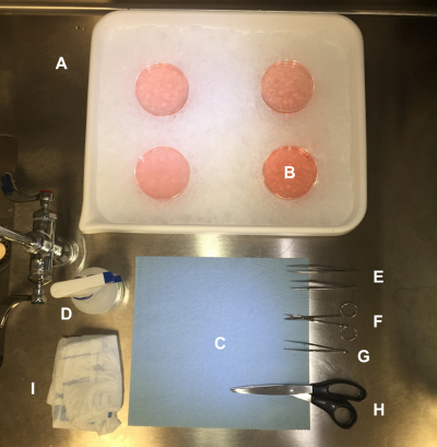
Figure 1: Tools and Materials used for Embryo Removal. (A) Ice-filled tray. (B) Petri dishes filled with cold L-15 "slush." (C) Paper towel. (D) Spray bottle with 70% ethanol. (E) Fine forceps (x2). (F) Small surgical scissors. (G) Blunt-nose thumb forceps. (H) Large scissors. (I) Body bag. Please click here to view a larger version of this figure.

Figure 2: Tools and Materials used for Brain Extraction. (A) Ice-filled tray. (B) Petri dish containing embryo heads. (C) Foil-covered centrifuge tube with storage medium. (D) Inverted glass Petri dish. (E) Autoclaved filter paper. (F) Beaker with 70% ethanol. (G) Plastic pipette. (H) Iris scissors. (I) Fine forceps. (J) Thin double-ended spatula. (K) Paper towel. Please click here to view a larger version of this figure.

Figure 3: Optimal versus Non-Optimal Cultures. (A) shows a healthy carpet of cells covering the arrays, in contrast to (B), in which there is poor cell proliferation. Please click here to view a larger version of this figure.

Figure 4: Representative Results of Spontaneous Activity. (A) Representative raster plot of spontaneous activity. The tick marks indicate action potentials recorded from 9 active electrodes during a 20 s window at an acquisition rate of 25 kHz and a bandpass filter range between 3 kHz and 300 Hz. (B) Representative filtered extracellular action potential from an active site. Figure modified from reference¹⁵. Please click here to view a larger version of this figure.

Figure 5: Recording Setup. (A) Stimulation generator. (B) Temperature controller. (C) Power supply. (D) Amplifier. (E) Headstage/preamplifier. (F) Capped MEA. Please click here to view a larger version of this figure.

Figure 6: Schematic Representation of the Electrical Training Protocol. Record an initial baseline for 5 min and a probe stimulation for 3 min. Apply tetanic stimulation for 90 s, which is not recorded. Apply and record a second probe stimulation for 3 min and a final baseline for 5 min. Please click here to view a larger version of this figure.

Figure 7: Probing Stimulation and Training Signal Parameters. (A) Probing stimulation consists of ±900 mV bi-phasic pulses administered at a frequency of 0.5 Hz. (B) Pulse trains consist of 100, ±900 mV bi-phasic pulses at a frequency of 250 Hz. (C) The training signal consists of 40 pulse trains administered every 2 s. Figure modified from reference¹⁵. Please click here to view a larger version of this figure.

Figure 8: Representation of the "L"-shape Configuration. Squares represent individual electrodes from an MEA. Blue squares indicate electrodes used for stimulation, whereas all others are used for recording. Figure modified from reference¹⁵. Please click here to view a larger version of this figure.

Figure 9: Distinguishing Units from Noise and Stimulation Artifacts. The several upper panels (A-C) in this figure show examples of noise in order to clarify what a "unit" should be. (D) The yellow waveform is the only unit detected here. (E) The green waveform is the only unit. (F) Example of a channel that was recorded from an electrode that was also used for stimulation, where no units can be reasonably detected due to amplifier saturation. Please click here to view a larger version of this figure.

Figure 10: Post-stimulus Time Histogram (PSTH). A graphical user interface (see Materials Table) plots the PSTHs according to user input (i.e., population PSTH, biased-average PSTH, or individual channel PSTH), allowing for an overview of the stimulation experiment and for immediate comparison between the post- and pre-stimulus files. It also plots the initial versus final PSTHs; this compares the network response to the first 6 and the last 6 stimuli. The GUI performs several other functions, such as spike rate, inter-spike interval, spikes per burst, inter-burst interval, and burst duration, for both stimulation files and files with spontaneous activity. Please click here to view a larger version of this figure.

Figure 11: Overview of Cell Preparation and Plating. (A) An E17 pregnant mouse is euthanized with CO₂. (B) The mouse is decapitated and the uterus is removed. (C) The embryos are released and decapitated. (D) The brain is extracted from each embryo and the frontal lobes are removed. (E) The cells are dissociated. (F) The dissociated cells are suspended in medium. (G) The suspended cells are plated on 60-channel multi-electrode arrays (MEAs). Please click here to view a larger version of this figure.

Figure 12: Neuronal Cultures Plated on Microelectrode Arrays. Embryonic mouse neurons are plated on 60-channel MEAs, which allow for the simultaneous recording of the neuronal activity across the network from each electrode. (Figure modified from reference¹⁵). Please click here to view a larger version of this figure.

Figure 13: Sorting Program used to Sort the Waveforms from Each Channel. The sorting program (see Materials Table) loads a data file and displays all the units initially acquired for each channel. One of several methods is selected to assign signals to specific units. In this example, the k-means clustering algorithm was selected, and the yellow unit (labeled "unit a" on the bottom window) was identified. Another program (see Materials Table) is then used to export the .nex file into a .mat file, which is the input file for the custom-made GUI (see Materials Table and Figure 10). Please click here to view a larger version of this figure.

Figure 14: Altered Network Activity in Response to Stimulation after a Training Period. Representative raster plot of activity from eight electrodes. The vertical red line indicates the time of the stimulus, and the black tick marks indicate action potentials. In pre-training (A), there is an immediate response to the stimulus pulse across channels. In post-training (B), the network exhibits a more prolonged activity response, as well as the immediate response to the stimulation¹⁵. Please click here to view a larger version of this figure.

Figure 15: Trained Networks have Significantly Altered Spike Frequencies. The frequency of the network spiking for the control networks is calculated by integrating the number of spikes over 50 ms immediately after each stimulation and dividing by that period. Shown is the average of 12 trained and 10 control networks (the error bars indicate the standard error of the mean). The asterisk (*) indicates a statistical difference (p-value <0.05) between the two datasets. Figure modified from reference¹⁵. Please click here to view a larger version of this figure.

Figure 16: Synaptically-mediated Responses are Significantly Modified in Trained Networks. (A) The spike reliability, measured in 10 ms bins and normalized to the control networks, shows no change for the direct activation of neurons near electrodes (0-20 ms). There is therefore no statistical difference between controls and trained networks for those bins. On the other hand, the longer-latency responses (30-50 ms), are synaptically mediated, indicating that this method provides a more detailed investigation of reliability than in Figure 15, above. (B) The population spike frequency repeats the behavior of the reliability and shows no modification for the direct activation (0-20 ms), while a statistically significant difference is found for the longer-term responses (30-50 ms). This behavior is consistent with the averaged results in the previous figure¹⁵. The error bars are the standard error of the mean, calculated for 10 control networks and 12 trained networks. (*) p-value <0.05; (**) p-value <0.001. Figure modified from reference¹⁵. Please click here to view a larger version of this figure.

Qty	Item
1	Autoclaved glass reagent bottle (at least 100 mL size)
20	15 mL sterile centrifuge tubes
1	10 mL sterile serological pipette
4	25 mL sterile serological pipette
2	50 mL sterile serological pipette
1	Centrifuge tube rack
150 mL	Sterile DI water
5 mg	Poly-D-lysine vial

Table 1: PDL Preparation - List of Materials and Reagents.

Qty	Item
1	50 mL sterile centrifuge tubes
10	15 mL sterile centrifuge tubes
2	1 mL sterile serological pipette
2	50 mL sterile serological pipette
1	Centrifuge tube rack
1 mL	Phosphate buffer saline (PBS)
1 mg	Laminin

Table 2: Laminin Preparation - List of Materials and Reagents.

Qty	Item
1	Autoclaved glass reagent bottle (at least 100 mL size)
20	15 mL sterile centrifuge tubes
1	10 mL sterile serological pipette
4	25 mL sterile serological pipette
2	50 mL sterile serological pipette
1	Centrifuge tube rack
150 mL	Sterile DI water
5 mg	Poly-D-lysine vial

Table 3: Storage Medium Preparation - List of Materials and Reagents.

Qty	Item
44 mL	DMEM with a stablilzed form of L-glutamine (see table of materials)
1 mL	Serum-free supplement for neural cell culture (see table of materials)
2.5 mL	Horse serum
100 µL	Ascorbic acid [4 mg/mL]
2.5 mL	Fetal bovine serum (FBS)
0.5 mL	Pen strep (optional)
1	50 mL sterile centrifuge tubes
2	25 mL sterile serological pipette
2	10 mL sterile serological pipette
2	1 mL sterile serological pipette
1	250 mL filter

Table 4: DMEM 5/5 Medium Preparation - List of Materials and Reagents.

Qty	Item
49 mL	DMEM with a stablilzed form of L-glutamine (see table of materials)
1 mL	Serum-free supplement for neural cell culture (see table of materials)
100 µL	Ascorbic acid [4 mg/mL]
0.5 mL	Pen strep (optional)
1	50 mL sterile centrifuge tubes
2	25 mL sterile serological pipette
2	1 mL sterile serological pipette
1	250 mL filter

Table 5: DMEM+ Medium Preparation - List of Materials and Reagents.

Qty	Item
1	Papain 140 U/vial
1	Dnase 1,260 U/vial
7 mL	DMEM+ (chilled)
5 mL	DMEM 5/5 (warmed)
10 µL	Trypan blue
2	Scalpel blades
1	35 mm sterile Petri dish
4	15 mL sterile centrifuge tubes
2	5 mL sterile cryogenic tubes
2	2 mL sterile cryogenic tubes
1	50 mL sterile centrifuge tubes
1	microcentrifuge tube
2	Large bore transfer pipette
3	Small bore transfer pipette
5	2 mL sterile serological pipette
5	1 mL sterile serological pipette
2	10 µL sterile micropipette tips
1	1000 µL sterile micropipette tips
1	Hemocytometer chip

Table 6: Cell Dissociation - List of Materials and Reagents.

Discussion

The steps outlined in this protocol provide sufficient detail for the beginner to plate his/her own neuronal cultures on MEAs and to record network activity. This protocol will help to ensure that the cultures adhere properly, forming a carpet layer of cells over the electrode arrays, and remain healthy and contaminant-free for months.

Although it is best to adhere to all parts of the protocol, there are steps throughout the process that are critical to the successful outcome. The use of aseptic technique throughout the entire process is imperative to prevent the cultures from becoming contaminated. New MEAs must be made hydrophilic, as described in the protocol, or else poor cell adhesion will result. Avoiding harsh pipetting and the formation of air bubbles during dissociation will reduce the number of damaged cells plated and will lead to a higher and healthier yield. Switching from DMEM 5/5 to DMEM+ after the first feeding is also important. DMEM 5/5 contains horse serum, which will cause glial cells to dominate the culture if used continuously and will result in poor neuronal activity, although the cultures will appear healthy¹⁷. Feeding the cultures as scheduled and keeping them in proper incubating conditions is also crucial.

Plating cell cultures on MEAs involves many variables that can lead to less-than-optimal results. Although the goal is a perfect "carpet" of cells, failure to address the critical steps mentioned above will result in poor cell maturation or in contamination. Poor cell adhesion, which is different from poor cell maturation, is also a concern. This can be caused by several factors, including poor MEA preparation prior to plating or the use of old medium. If old medium containing a stabilized form of L-glutamine and serum-free supplement for neural cell culture (see Materials Table) is used, the cells initially adhere but then float away after about two weeks. If bacterial contamination is a persistent problem, an antibiotic, such as ampicillin or pen-strep, can be added to the medium. There are also fungicides available to treat fungal contamination. These are some of the more common variables that can affect the outcome of the cultures. There are many others that will only be encountered after time and experience.

In comparison to the use of glass microelectrodes, this technique is excellent for studying network dynamics and pharmacological responses. It enables the use of many different spatio-temporal stimulation patterns and allows for the recording of neuronal responses from multiple areas at once. Previous groups have demonstrated interesting results using protocols similar to the ones described here¹⁸. Since the cultures last for weeks or months and the same cultures can be reused, this technique also allows for multiple experiments over time on the same network.

However, there are limitations to this technique. MEAs are non-invasive. Therefore, they can only record extracellular activity, as opposed to patch-clamping or intracellular recording with pipettes. Moreover, since each electrode in an array is covered by several cells, it is not possible to resolve the activity of a single neuron. Conversely, because these are in vitro cultures, they cannot fully reproduce the structural properties of networks in the brain. Also, activity can only be recorded for less than 30 min at a time without some mechanism providing a CO₂ atmosphere for the cells to maintain their pH balance.

Once this technique is mastered,pharmacological manipulations with or without electrical stimulation can be explored. New protocols to probe learning and memory formation in neuronal networks can also be designed and tested, along with protocols for hippocampal or spinal cord networks. Protocols for the stimulation and training of networks have been previously published, and some of these were further developed into in vivo protocols, such as the "selective adaptation" proposed by Eytan et al.¹⁹. Several protocols were tested. However, only results from a modification to the tetanus procedure proposed by Ruaro in 2005 are presented here^14,20.

Materials

List of materials used in this article

Name	Company	Catalog Number	Comments
Ascorbic Acid	Sigma Aldrich	A4403	Make 4 mg/mL aliquots
B-27	Invitrogen	17504-044	Serum-free supplement for neural cell culture. Make 1 mL aliquots and freeze
Beakers - glass - 100 mL	VWR	13912-160
Beakers - glass - 500 mL	VWR	10754-956
Blunt-tipped thumb forceps	World Precision Instruments	500365-G
Cryogenic vial - sterile, 2 mL	Fisher Scientific	10-500-26
Cryogenic vial - sterile, 5 mL	Fisher Scientific	10-500-27
DMEM with Glutamax	Gibco Life Technology	10569-010	Cell culture media that contains a stabilized form of L-glutamine
DNase	Worthington Biochemical	LK003172
Ethanol	Fisher Scientific	04-355-451
Fetal bovine serum (FBS)	ATCC	30-2030
Fine-tipped thumb forceps	World Precision Instruments	501324-G
Glass Pipets	VWR	14673-010
GlutaMAX -- I (100X)	Gibco Life Technology	35050-061	A stabilized form of L-glutamine used as a suplement
Hemocytometer chip	Fisher Scientific	22-600-101
Hibernate EB complete	BrainBits	D00118	Ambient CO2 cell storage media
Horse Serum	Atlanta Biologicals	S12195H
Laminin	Sigma Aldrich	L2020-1MG
MCS filter amplifier	MultiChannel System	FA60SBC
MCS headstage/pre-amplifier	MultiChannel System	MEA1060-INV
MCS microelectrode array	MultiChannel System	60MEA200/10iR-ITO
MCS power supply	MultiChannel System	PS20W
MCS signal divider	MultiChannel System	SDMEA
MCS stimulus generator	MultiChannel System	STG4002
MCS temperature controller	MultiChannel System	TC02
Media storage bottle - glass 500 mL	VWR	10754-818	Autoclave
Microcentrifuge tubes - 0.4 mL	Thermo Fisher	3485	Autoclave
Microcentrifuge tubes - 2 mL	Thermo Fisher	3434ECONO	Autoclave
Micropipette tips - 10 μL	VWR	37001-166	Autoclave
Micropipette tips - 1,000 μL	VWR	13503-464	Autoclave
Micropipette tips - 200 μL	VWR	37001-596	Autoclave
Micropipetter - 10 μL	Thermo Fisher	4641170N
Micropipetter - 1,000 μL	Thermo Fisher	4641210N
Micropipetter - 200 μL	Thermo Fisher	4641230N
Papain - 0.22 Filtered	Worthington Biochemical	LK003178
Penicillin-Streptomycin (Pen Strep)	Thermo Fisher	15070063
Petri dishes -100 mm disposable	Fisher Scientific	08-757-100D
Petri dishes -100 mm glass	VWR	10754-788
Petri dishes -35 mm	Fisher Scientific	08-757-100A
Phosphate buffer saline (PBS) (1x)	Corning	21-040-CV
Plasma Cleaning System	Plasma Etch, Inc.	PE-50
Poly-D-lysine hydrobromide (PDL)	Sigma Aldrich	P6407-5MG
Polyethylene conical (centrifuge) tube -15 mL	Fisher Scientific	05-527-90
Polypropylene conical (centrifuge) tube -50 mL	Falcon	352070
Procedure masks	Imco	1530-imc
Pyruvate	Sigma Aldrich	P4562-5G
Scalpel blades	World Precision Instruments	500237-G
Scissors - iris	World Precision Instruments	14111-G
Scissors - large	World Precision Instruments	14214
Scissors - small surgical	World Precision Instruments	501733-G
Serological pipette - sterile, 1 mL	VWR	89130-892
Serological pipette - sterile, 2 mL	VWR	89130-894
Serological pipette - sterile, 25 mL	VWR	89130-900
Serological pipette - sterile, 50 mL	VWR	89130-902
Software: Matlab GUI	Peixoto Lab	npeixoto@gmu.edu	Used to analyze .mat files.  Available for free upon request.  Contact npeixoto@gmu.edu to request a copy.
Software: MCS MC_Rack	MultiChannel System	N/A	Used for data acquisition
Software: NeuroExplorer	Plexon	http://www.plexon.com/products/neuroexplorer	Used to convert .nex files to .mat
Software: Offline Sorter	Plexon	http://www.plexon.com/products/offline-sorter	Used to sort neural spikes and convert data files to .plx and then to .nex
Software Manual: MCS MC_Rack	MultiChannel System		https://www.multichannelsystems.com/sites/multichannelsystems.com/files/documents/manuals/MC_Rack_Manual.pdf
Software Manual: NeuroExplorer	Plexon		https://www.neuroexplorer.com/downloads/Nex3Manual.pdf
Software Manual: Offline Sorter	Plexon		www.plexon.com/system/files/downloads/Offline%20Sorter%20v2.8%20Manual.pdf
Spatula - small double-ended	World Precision Instruments	503440
Stericup 0.22 µm pore filter - 250 mL	Millipore	SCGVU02RE
Transfer pipette - large bore	Thermo Fisher	335-1S
Transfer pipette - small bore	Thermo Fisher	242-1S
Trypan blue	Sigma Aldrich	T8154-20ML
Whatman filter paper	Whatman	1442 150	Cut into 8 pie wedges and autoclave in a glass Petri dish

References

- Charkhkar, H., Frewin, C., et al. Use of cortical neuronal networks for in vitro material biocompatibility testing. Biosens Bioelectron. 53, 316-323 (2014).
- Bologna, L. L., Nieus, T., Tedesco, M., Chiappalone, M., Benfenati, F., Martinoia, S. Low-frequency stimulation enhances burst activity in cortical cultures during development. Neuroscience. 165 (3), 692-704 (2010).
- Fröhlich, F., McCormick, D. A. Endogenous electric fields may guide neocortical network activity. Neuron. 67 (1), 129-143 (2010).
- Anastassiou, C. A., Perin, R., Markram, H., Koch, C. Ephaptic coupling of cortical neurons. Nature Neurosci. 14 (2), 217-223 (2011).
- Ozen, S., Sirota, A., et al. Transcranial electric stimulation entrains cortical neuronal populations in rats. J. Neurosci. 30 (34), 11476-11485 (2010).
- Wagenaar, D. A., Madhavan, R., Pine, J., Potter, S. M. Controlling bursting in cortical cultures with closed-loop multi-electrode stimulation. J. Neurosci. 25 (3), 680-688 (2005).
- Shahaf, G., Marom, S. Learning in networks of cortical neurons. J. Neurosci. 21 (22), 8782-8788 (2001).
- Marom, S., Shahaf, G. Development, learning and memory in large random networks of cortical neurons: lessons beyond anatomy. Q Rev Biophys. 35 (1), 63-87 (2002).
- Marom, S., Eytan, D. Learning in ex-vivo developing networks of cortical neurons. Prog Brain Res. 147, 189-199 (2005).
- Li, Y., Zhou, W., Li, X., Zeng, S., Luo, Q. Dynamics of learning in cultured neuronal networks with antagonists of glutamate receptors. Biophys. J. 93 (12), 4151-4158 (2007).
- Li, Y., Zhou, W., Li, X., Zeng, S., Liu, M., Luo, Q. Characterization of synchronized bursts in cultured hippocampal neuronal networks with learning training on microelectrode arrays. Biosens Bioelectron. 22 (12), 2976-2982 (2007).
- Chiappalone, M., Massobrio, P., Martinoia, S. Network plasticity in cortical assemblies. Eur. J. Neurosci. 28 (1), 221-237 (2008).
- le Feber, J., Stegenga, J., Rutten, W. L. C. The effect of slow electrical stimuli to achieve learning in cultured networks of rat cortical neurons. PloS one. 5 (1), 8871(2010).
- Ruaro, M. E., Bonifazi, P., Torre, V. Toward the neurocomputer: image processing and pattern recognition with neuronal cultures. IEEE Trans Biomed Eng. 52 (3), 371-383 (2005).
- Hamilton, F., Graham, R., et al. Time-Dependent Increase in Network Response to Stimulation. PloS one. 10 (11), 0142399(2015).
- Guidelines for Euthanasia of Rodents Using Carbon Dioxide. , Available from: https://oacu.oir.nih.gov/sites/default/files/uploads/arac-guidelines/rodent_euthanasia_adult.pdf (2016).
- Banker, G., Goslin, K. Culturing Nerve Cells: Business Source. , MIT Press. Cambridge. (1998).
- Gullo, F., Maffezzoli, A., Dossi, E., Wanke, E. Short-latency cross-and autocorrelation identify clusters of interacting cortical neurons recorded from multi-electrode array. J. Neurosci. Methods. 181, 186-198 (2009).
- Eytan, D., Brenner, N., Marom, S. Selective Adaptation in Networks of Cortical Neurons. J. Neurosci. 23 (28), (2003).
- Bonifazi, P., Ruaro, M. E., Torre, V. Statistical properties of information processing in neuronal networks. Eur. J. Neurosci. 22 (11), 2953-2964 (2005).
Reprints and Permissions