Real-time Electrophysiology: Using Closed-loop Protocols to Probe Neuronal Dynamics and Beyond

Summary

Closed-loop protocols are becoming increasingly widespread in modern day electrophysiology. We present a simple, versatile and inexpensive way to perform complex electrophysiological protocols in cortical pyramidal neurons in vitro, using a desktop computer and a digital acquisition board.

Abstract

Experimental neuroscience is witnessing an increased interest in the development and application of novel and often complex, closed-loop protocols, where the stimulus applied depends in real-time on the response of the system. Recent applications range from the implementation of virtual reality systems for studying motor responses both in mice¹ and in zebrafish², to control of seizures following cortical stroke using optogenetics³. A key advantage of closed-loop techniques resides in the capability of probing higher dimensional properties that are not directly accessible or that depend on multiple variables, such as neuronal excitability⁴ and reliability, while at the same time maximizing the experimental throughput. In this contribution and in the context of cellular electrophysiology, we describe how to apply a variety of closed-loop protocols to the study of the response properties of pyramidal cortical neurons, recorded intracellularly with the patch clamp technique in acute brain slices from the somatosensory cortex of juvenile rats. As no commercially available or open source software provides all the features required for efficiently performing the experiments described here, a new software toolbox called LCG⁵ was developed, whose modular structure maximizes reuse of computer code and facilitates the implementation of novel experimental paradigms. Stimulation waveforms are specified using a compact meta-description and full experimental protocols are described in text-based configuration files. Additionally, LCG has a command-line interface that is suited for repetition of trials and automation of experimental protocols.

Introduction

In recent years, cellular electrophysiology has evolved from the traditional open-loop paradigm employed in voltage and current clamp experiments to modern closed-loop protocols. The best known closed-loop technique is perhaps the dynamic clamp^6,7, which enabled the synthetic injection of artificial voltage-gated ion channels to determine the neuronal membrane voltage⁸, the in-depth study of the effects of non-deterministic flickering on ion channels on neuronal response dynamics⁹, as well as the recreation in vitro of realistic in vivo-like synaptic background activity¹⁰.

Other closed-loop paradigms that have been proposed include the reactive clamp¹¹, to study in vitro the generation of self-sustained persistent activity, and the response clamp^4,12, to investigate the cellular mechanisms underlying neuronal excitability.

Here we describe a powerful framework that allows applying a variety of closed-loop electrophysiological protocols in the context of whole-cell patch clamp recordings performed in acute brain slices. We show how to record somatic membrane voltage by means of patch clamp recordings in pyramidal neurons from the somatosensory cortex of juvenile rats and apply three different closed-loop protocols using LCG, a command-line-based software toolbox developed in the laboratory of Theoretical Neurobiology and Neuroengineering.

Briefly, the described protocols are, first the automated injection of a series of current clamp stimulus waveforms, relevant for the characterization of a large set of active and passive membrane properties. These have been suggested to capture the electrophysiological phenotype of a cell in terms of its response properties to a stereotyped series of stimulus waveforms. Known as the e-code of a cell (e.g., see ^13,14), such a collection of electrical responses is used by several laboratories to objectively classify neurons on the basis of their electrical properties. This includes the analysis of the stationary input-output transfer relationship (f-I curve), by an innovative technique that involves the closed-loop, real-time control of the rate of firing by means of a proportional-integral-derivative (PID) controller, second the recreation of realistic in vivo-like background synaptic activity in in vitro preparations¹⁰ and , third the artificial connection in real-time of two simultaneously recorded pyramidal neurons by means of a virtual GABAergic interneuron, which is simulated by the computer.

Additionally, LCG implements the technique known as Active Electrode Compensation (AEC)¹⁵, which allows implementing dynamic clamp protocols using a single electrode. This allows compensating undesired effects (artifacts) of the recording electrode that arise when it is used for delivering intracellular stimuli. The method is based on a non-parametric estimate of the equivalent electrical properties of the recording circuit.

The techniques and experimental protocols described in this paper can be readily applied in conventional open-loop voltage and current clamp experiments and can be extended to other preparations, such as extracellular^4,16 or intracellular recordings in vivo^17,18. The careful assembly of the setup for whole cell patch clamp electrophysiology is a very important step for stable, high quality recordings. In the following we assume that such an experimental setup is already available to the experimenter, and focus our attention on describing the usage of LCG. The reader is pointed to ^19–22 for additional tips about optimization and debugging.

Protocol

The protocol described here complies with the recommendations and guidelines of the Ethics Committee of the Department of Biomedical Sciences of the University of Antwerp. This protocol requires the preparation of non-sentient material from the explanted brain of juvenile Wistar rats, obtained by approved humane euthanasia techniques.

1. Equipment Preparation

1. Install and configure the data acquisition and stimulation system.
   1. Use a personal computer (PC) equipped with a data acquisition (DAQ) card supported by Comedi to record signals and send analog control voltages to the electrophysiological amplifier.
      NOTE: Comedi is a Linux module and library that supports a multitude of DAQ cards from the most common manufacturers: visit http://www.comedi.org for more information.
   2. In case a computer-controlled patch clamp amplifier is in use, employ a second PC besides the one dedicated to the amplifier control.
      NOTE: While the latter may run a conventional operating system, the extra PC will be operating in real-time by means of a special operating system. Under these conditions, it is convenient to use a single monitor, mouse, and keyboard attached to the extra PC, while connecting by a remote desktop application to the dedicated PC.
   3. Download the ISO image of the Live CD containing a real-time Linux operating system with LCG preinstalled from http://www.tnb.ua.ac.be/software/LCG_Live_CD.iso and burn it on a blank CD or USB stick”.
   4. Simply insert the CD into the drive of the PC containing the DAQ card and start it. Alternatively, install LCG from its online source repository on a PC running the Linux operating system (e.g., Debian or Ubuntu). Consult the online manual for details on the installation procedure. The manual is available online at http://danielelinaro.github.io/dynclamp/lcg_manual.pdf.
   5. Boot from the live CD: this will automatically load a fully configured system. To do this, place the LCG Live CD in the computer CD-ROM drive and boot the computer from CD; select the real-time kernel (default option) as soon as the boot menu appears and wait for the system to initialize.
   6. Calibrate the DAQ card by typing at the command prompt:
      sudo comedi_calibrate
      or
      sudo comedi_soft_calibrate
      depending on whether the data-acquisition board supports hardware or software calibration, respectively (use the command sudo comedi_board_info to obtain information on the board).
   7. Set the appropriate analog-to-digital and digital-to-analog conversion factors: this requires having access to the manual of the cellular electrophysiological amplifier, and particularly to its specifications on its conversion factors.
   8. Use a text editor to specify the appropriate numerical values in the file /home/user/.lcg-env, for the environment variables AI_CONVERSION_FACTOR_CC, AI_CONVERSION_FACTOR_VC, AO_CONVERSION_FACTOR_CC, AO_CONVERSION_FACTOR_VC.
      NOTE: These represent the input (AI) and output (AO) gains for current clamp (CC) and voltage clamp (VC) modes, and the conversion factors between the voltage commands provided by the computer and the current or voltages generated by the amplifier, respectively.
   9. Alternatively, use the LCG script provided (lcg-find-conversion-factors), to find the conversion factors of his or her system.
      NOTE: The values computed by lcg-find-conversion-factors are guesses, which in some cases are required to be numerically truncated or rounded to reflect the exact values of the conversion factors.
   10. To use lcg-find-conversion-factors, start by connecting the 'model cell' that often is purchased with the amplifier to the corresponding headstage. Then, open a terminal on the Linux machine where you are running the Live CD and enter the following command at the shell prompt:
       lcg-find-conversion-factors -i $HOME/.lcg-env -o $HOME/.lcg-env 
       NOTE: In both cases (i.e., manual modification of /home/user/.lcg-env or usage of lcg-find-conversion-factors), close and open the terminal for the changes to take effect.
   11. If multiple headstages are used, set the conversion factors to the same values in all channels; if that is not possible, consult the LCG online manual to understand how to use multiple conversion factors in lcg-stimulus or how to produce configuration files that better suit the user’s needs.

2. Preparation of Acute Brain Slices from the Somatosensory Cortex

1. Preparation of solutions for electrophysiology.
   1. Prepare Artificial Cerebro-Spinal Fluid (ACSF) by mixing (in mM) 125 NaCl, 2.5 KCl, 1.25 NaH₂PO₄, 26 NaHCO₃, 25 glucose, 2 CaCl₂, and 1 MgCl₂. Prepare 10x stock solutions to reduce the preparation time on the day of the experiment. Prepare 2 L, of which one will be used for the preparation of the slices and the other for recording.
   2. Saturate the ACSF with 95% O₂ and 5% CO₂ for at least 30 min prior to the beginning of the procedure.
   3. For current clamp recordings, use an intracellular solution (ICS) containing (in mM) 115 K-gluconate, 20 KCl, 10 HEPES, 4 ATP-Mg, 0.3 Na₂-GTP, 10 Na₂-phosphocreatine. Prepare the solution in ice and filter it prior to the beginning of the recordings to eliminate the risk of clogging the pipette.
2. Brain extraction.
   1. Anesthetize the animal placing the animal in an induction chamber with 4% Isoflurane and rapidly decapitate it using a guillotine or large scissors.
   2. Cut the skin along the midline and slide it to the ears.
   3. Using a fine pair of scissors cut the skull along the midline. Keep the blade as close as possible to the surface so as to minimize damage to the underlying brain. Open the skull with a pair of tweezers, use a spatula to sever the optic nerve and the brainstem and gently drop the brain in ice-cold ACSF.
   4. Separate the cerebellum and the two hemispheres with a scalpel (blade 24).
   5. Remove excess water from one of the two hemispheres and glue it on an inclined platform using a drop of superglue. Quickly add a few drops of ACSF over the brain and transfer it to the vibratome chamber.
      NOTE: When preparing sagittal slices, the angle of the platform is important to avoid damaging the dendrites of pyramidal cells during the slicing procedure.
3. Preparation of the slices.
   1. Position the blade over the brain and discard the first 2.5 - 3 mm. Adjust the speed and frequency to limit damage to the surface of the slice while at the same time minimizing the time required for the slicing procedure.
   2. Set the thickness to 300 µm and begin slicing. Once the blade has gone past the cortex, use a razor blade or a bent needle to cut above the hippocampus and at the edges of the cortical area of interest.
   3. Place the slices in a multi-well incubation chamber kept at 32 - 34 °C.
   4. Retract the blade and repeat points 2.3.2 and 2.3.3 until 5 - 8 slices are cut. The best slices are usually the ones where the blood vessels are parallel to the surface.
   5. Incubate the slices for 30 min after the last slice is placed in the chamber.

3. Patch-clamp Recordings from Layer 5 Pyramidal Neurons

1. Place a slice in the recording chamber and search for healthy cells. These cells usually have lower contrast, a smooth appearance and are not swollen.
2. Inspect the slice under the microscope with the 40X magnification lens and search for cells in layer 5, located approximately 600 to 1,000 µm from the surface of the brain.
3. Once a suitable cell is found, load one third of the micropipette with ICS and place it in the headstage.
4. On the personal computer running the live CD or the pre-configured Linux operating system, launch a command shell (e.g., bash) and at its prompt type the command lcg-zero. This ensures that the DAQ board is not driving the amplifier.
5. Apply 30 - 50 mbar of positive pressure by pressing on the piston of a common syringe, connected by tubing to the pipette holder and, with the help of the microscope, place the pipette approximately 100 µm above the slice.
   NOTE: Place the pipette in a position that allows a direct route to the target cell, preferably using the approach mode of the micromanipulator.
6. Acting on the controls the electrophysiology amplifier, adjust the pipette offset and output a test pulse (10 mV) in voltage clamp mode.
7. Reduce the pressure to 10 - 30 mbar (depending on the pipette size) by withdrawing the piston of the syringe; gently approach the cell and check for the formation of a dimple by observing the image on the video camera monitor. Monitor the test pulse for an increase in resistance at all times, by watching the current waveform displayed on the oscilloscope connected to the electrophysiology amplifier (alternatively you can use the command lcg-seal-test to monitor the pipette resistance).
8. Release the pressure and if necessary apply gentle negative pressure to the pipette to help seal formation when you notice an increase in pipette resistance and the formation of a 'dimple' on the cell.
9. While the seal forms, gradually decrease the holding potential to -70 mV.
10. Once a gigaohm seal has been obtained, ensure that the holding current is between 0 - 30 pA. Apply short pulses of negative pressure (suction) to break the membrane and establish the whole-cell configuration. Alternatively, you can inject strong and brief pulses of voltage (i.e., using the 'ZAP' command on the amplifier or holding the cell at very negative) to rupture the membrane, depending on the preparation and glass pipette used.
11. Switch to current clamp mode and verify that the resting membrane potential is typical of a healthy cell. For cortical pyramidal neurons using a potassium-gluconate-based solution, this value is usually between -65 and -75 mV.

4. Semi-automatic Characterization of a Neuron’s Electrical Response Properties

1. Create a directory to store user’s data. In order to do this the employ a script included in the LCG live CD that creates folders based on the date. To use it, type at the command prompt
   cd ~/experiments
   lcg-create-experiment-folder -s psp,in_vivo_like
   This will create a folder where the data for that cell will be saved (and a 'psp' and 'in_vivo_like' subfolders) and it will print its name to the terminal window; it is also possible to store additional information such as pipette resistance and cell type using this script.
2. Change directory to the newly created folder using the command
   cd ~/<foldername>
   The folder name is the one displayed by the command lcg-create-experiment-folder and will have the timestamp of the current day (i.e., year-month-day), as in 20140331A01.
3. Make sure that the amplifier is set to operate in current clamp mode, that the cables are connected and the external voltage command of the amplifier, if present, is enabled.
4. Enter the command lcg-ecodeat the command prompt. This calls a series of commands (namely lcg-ap, lcg-vi, lcg-ramp, lcg-tau and lcg-steps), used to characterize basic response properties of the cell. lcg-ecode requires that the user specify two parameters: the amplitude of the 1 ms-long pulse of current used to elicit a single spike in the cell, and the maximum amplitude of the current ramp injected into the cell to find its rheobase.
   Use the following command syntax:
   lcg-ecode --pulse-amplitude X --ramp-amplitude Y
   with a choice of the values X and Y (in pA) that are sufficient to make the cell fire in response to a 1 ms-long pulse and a sustained injection of current, respectively.
   NOTE: These protocols require performing the numerical estimate of the 'electrode kernel' in order to use the Active Electrode Compensation (AEC)¹⁵. A noisy current injection is used to estimate the kernel and the user is prompted to confirm the number of samples that make up the kernel. See ¹⁵ for detailed information on the meaning of the electrode kernel and how to choose the number of kernel samples.

5. Injection of Conductance through Simulated Synapses and Simulation of In Vivo-like Background Activity

1. Injection of simulated excitatory post-synaptic potentials
   1. Change to the directory where you will save the next experiment, by typing the following command at the command prompt of the shell:
      cd psp/01
   2. Copy an LCG configuration file to the current directory and open it with a text editor (Nano in this example) by typing the following commands at the command prompt of the shell (this example configuration file is included in the source code and the live cd):
      cp ~/local/src/lcg/configurations/epsp.xml 
      nano epsp.xml
      NOTE: This is simply a text file with different entities connected to each other. For more details see the Representative Results section.
   3. If necessary edit the inputChannel, outputChannel, the inputConversionFactor and the outputConversionFactor in this file to match the user’s setup.
   4. Compute the electrode kernel needed to perform the active electrode compensation ' the method used by LCG to perform single electrode dynamic clamp ' by issuing the command
      lcg-kernel
      This will prompt for the number of points in the kernel. Again, select a number so that the electrode kernel covers the end of the exponential decay tail.
   5. Perform the dynamic clamp experiment using the command
      lcg-experiment -c epsp.xml
   6. List the files and visualize the results by using the command
      ls -l
      lcg-plot-file -f last
2. Injection of simulated inhibitory post-synaptic potentials
   1. Create a folder and copy the epsp.xml file to it by typing the following commands at the command prompt of the shell:
      mkdir ../02
      cp epsp.xml ../02/ipsp.xml
      cd ../02
   2. Edit the configuration file by using a text editor: change the synaptic reversal potential and rise and decay time constants of the model synapse Exp2Synapse to the following:
      parameters>
      <E>-80</E>
      <tauRise>0.8e-3</tauRise>
      <tauDecay>10e-3</tauDecay>
      <parameters>
      Quit the text editor.
   3. Compute the electrode kernel and perform the experiment as in 5.1, by typing the following commands at the command prompt of the shell:
      lcg-kernel
      lcg-experiment -c ipsp.xml
   4. List the files and visualize the results, by typing the following commands at the command prompt of the shell:
      ls -l
      lcg-plot-file -f <filename.h5>
3. Simulation of in vivo-like background activity:
   1. Change to the directory where you want to save the following experiment, as previously shown, by typing the following commands at the command prompt of the shell:
      cd ../../in_vivo_like/01
   2. Copy the configuration file from LCG source directory, by typing the following commands at the command prompt of the shell:
      cp ~/local/src/lcg/configurations/in_vivo_like.xml 
      nano in_vivo_like.xml
      NOTE: This file is simply the concatenation of the previous ones; two Poisson-point processes that generate spike trains, which in turn feed inhibitory and excitatory model synapses, generate the background activity.
   3. Adjust the DAQ configuration parameters for the user’s setup, as described in 5.1.3 and exit the editor.
   4. Compute the electrode kernel and perform the experiment as in 5.1, by typing the following commands at the command prompt of the shell:
      lcg-kernel
      lcg-experiment -c in_vivo_like.xml -n 10 -i 3
      The '-n 10' and '-i 3' switches indicate that the stimulation should be repeated 10 times at intervals of three sec.
   5. Visualize the raw traces by using the following command at the command prompt of the shell:
      lcg-plot-file -f all

Results

In the previous sections, we have described how to use the software toolbox LCG to characterize the electrophysiological properties of L5 pyramidal cells and to recreate in vivo-like synaptic activity in a slice preparation. The use of a command-line interface and semi-automated protocol favor the reproducibility and efficiency of the experiment, which can have a large impact on the output and quality of the data produced. Additionally, since the data is saved in a consistent way, it is easy to extend the analysis to a particular goal. Figure 1 shows the typical result of an experiment in which basic electrophysiological properties of a cell using six distinct protocols have been characterized.

Measurement of action potential shape and threshold (Figure 1A): a brief and strong pulse of depolarizing current is injected to measure the average action potential shape. The spike threshold is computed as the first peak of the third derivative of the action potential²⁴. Measurement of the voltage-current curve (Figure 1B): sub-threshold current pulses are injected into the cell, allowing the measurement of passive response properties such as input resistance and the characterization of sub-threshold ionic currents.

Measurement of the minimal current sufficient for eliciting sustained firing (Figure 1C). The injected ramp of current allows for characterization of the cell as a type I or type II oscillator²⁵. Measurement of the frequency-current (f-I) curve (Figure 1D): the injected current is a function of the instantaneous firing frequency and is updated every time the cell spikes, using the closed-loop protocol described in ⁵. Using this technique, a reliable estimation of the f-I curve can be obtained in less than 30 sec. Measurement of the membrane time constant (Figure 1E): a short hyperpolarizing current pulse is delivered to measure the passive relaxation properties of the membrane. This pulse is then fit to a double exponential to compute the membrane time constant (44 ms in this case).

Adaptation coefficient and response to depolarizing current (Figure 1F): two supra-threshold values of current are injected to measure the adaptation coefficient (ratio between the first and last inter-spike intervals). The automated application of a series of protocols like the ones described allows characterizing each recorded cell in terms of its key electrophysiological properties and constitutes the basic step for any effort aimed at comparing different neuron types and their role, both in health and disease.

Although LCG contains several scripts that implement specialized protocols, most of the power and flexibility of the toolbox resides in the ability to describe experiments by means of configuration files. In Sec. 5 it is described how to perform dynamic clamp to inject simulated background activity into the neuron. Here the concept of configuration files and entities is introduced. A configuration file is simply a text file containing the names and interconnections of all the basic building blocks (called entities) that are required for performing a given experiment; for this reason, designing novel paradigms by connecting entities is a relatively easy task, as is sharing and reusing experimental paradigms. In the experiment shown in Figure 2, five entities are used:

H5Recorder: records the connected entities to a compressed file. The HDF5 file format has been chosen since it is supported by most programming languages such as Python and MATLAB.

RealNeuron: provides an abstraction layer to the technical aspect of the real-time recording and injection. It contains the information about the data acquisition board and performs the active electrode compensation online. When an action potential is detected by threshold crossing, Real Neuron also outputs a spike in the form of an event: this can be used for instance to monitor the firing rate during the experiment or to interface with artificial synapses.

Poisson: generates spike trains following an exponential distribution with a particular rate. The seed of this process can be fixed so that trials can be reproduced consistently.

SynapticConnection: receives the spikes from the generator and relays them to the appropriate synapse after a given delay.

Exp2Synapse: model of a double exponential synapse. It contains the reversal potential and the rise and decay time constants.

As mentioned previously, each entity is connected to one or more others to compose an experiment. In the example of the simulation of an excitatory post-synaptic current described in Sec. 5.1, both the RealNeuron and the Exp2Synapse are connected to the H5Recorder, to save to file membrane voltage and synaptic current, respectively. The Poisson entity delivers spikes generated at a frequency of 2 Hz to the SynapticConnection, which in turn delivers the events to the Exp2Synapse after 1 ms. Finally, the Exp2Synapse entity is connected to the RealNeuron. Using small variations of this configuration file, as shown in Secs. 5.2 and 5.3, one can simulate inhibitory currents and recreate in vivo-like activity.

In Figure 2 it is shown how, by means of a dynamic clamp configuration, one can study synaptic integration in a controlled fashion by simulating the current induced into a neuron by artificial synapses. Figure 2A (top) shows individual post-synaptic potentials (top) together with the injected currents. Red (blue) traces denote excitatory (inhibitory) events. Note that the injected current is a function of the membrane voltage and of the change in conductance associated to the activation of the virtual synapse.

By delivering Poisson spike trains at higher frequencies to the synapses, in vivo-like background activity can be simulated (Figure 2B and 2D). Even during spiking when large currents are injected (black trace in the bottom of Figure 2B), the Active Electrode Compensation guarantees that the shape of the spikes is not affected (Figure 2C), even though a single electrode is used to simultaneously inject current and record the membrane voltage. Repeating multiple trials with the same conductance waveforms allows extending the work of ²³ to a more realistic framework, making it possible to separate the contributions of different synaptic currents to reliability and precision of spike timing.

Figure 3 shows a simple example of hybrid network, obtained by recording simultaneously from two unconnected pyramidal cells and using a virtual GABAergic interneuron to simulate a form of disynaptic inhibition, a widespread mechanism that in the cerebral cortex involves the activation of Martinotti cells.^26,27 Figure 3A shows a schematic of the experimental setup: a pair of real, unconnected pyramidal cells (black and red triangles) is artificially connected through a simulated GABAergic interneuron, modeled as a leaky integrate-and-fire neuron. The synapse that connects the presynaptic pyramidal cell to the interneuron displays homosynaptic short term facilitation implemented according to the Tsodyks-Markram model²⁸, while the synapse connecting the interneuron and the postsynaptic pyramidal cell is a biexponential synapse with rise and decay time constants of 1 and 10 ms, respectively.

The weights of both connections were adjusted to have a deflection in the postsynaptic membrane potential of approximately 2 mV. Figure 3B and 3C show the response of the presynaptic pyramidal neuron to a train of intracellular pulses delivered at 90 Hz and the corresponding EPSPs in the simulated interneuron: the parameters of the synaptic connection were adjusted in order to have the artificial neuron emit a spike after a presynaptic burst of 3 - 4 spikes at high frequency, as reported experimentally.^26,29 Figure 3D shows the effect of the disynaptic inhibition on the real postsynaptic pyramidal cell: 10 trials are superimposed, in which the neuron is stimulated with frozen in vivo-like background activity similar to the one described in Figure 2. Note the increase in reliability in response to the three inhibitory IPSPs, reflected in the smaller spike jitter after the activation of the inhibitory cell, as indicated by the red dashes below the voltage traces.

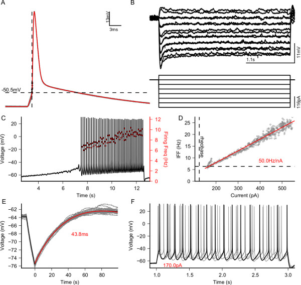
Figure 1. Electrophysiological characterization of a patched L5 Pyramidal neuron. Output figure of the e-code protocol for a typical pyramidal cell; quantifications are performed automatically and no further editing is required. (A) Calculation of action potential threshold (dashed line -50.5 mV). Red line is the average action potential shape. (B) Measurement of passive response (top) to hyperpolarizing currents (bottom). (C)  Response to an increasing depolarizing current to measure the rheobase current (123 pA). (D) Firing frequency as a function of the injected current, measured using a closed-loop approach. Each gray point is located at the pair (current injected, inverse of the interspike interval). The red curve is the linear fit to the data points and the dashed line indicates the rheobase measured in panel (C). (E) Measure of the membrane time constant (43.8 ms). (F) Identification of basic active properties of the cell reveals that the cell is a regular spiking neuron and that there is minimal adaptation. Please click here to view a larger version of this figure.

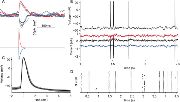
Figure 2. Recreation of in vivo-like activity using dynamic clamp. (A) Simulation of excitatory (red, Sec. 5.1) and inhibitory (blue, Sec. 5.2) synapses, gray traces are other realizations of the same experiment. (B)  Top, voltage traces recorded from a L5 pyramidal neuron subject to a bombardment of excitatory (inhibitory) post-synaptic currents at a rate of 7,000 (3,000) Hz. Multiple realizations with a fixed random seed are displayed in the figure (grey traces). Bottom, corresponding excitatory (red), inhibitory (blue) and total (black) current injected into the cell. (C) Shapes of the spikes during the experiment in (B). (D) Raster plot of the spikes generated across 20 trials shows that the neuron can be extremely reliable and precise in response to the same input as seen in ²³. Please click here to view a larger version of this figure.

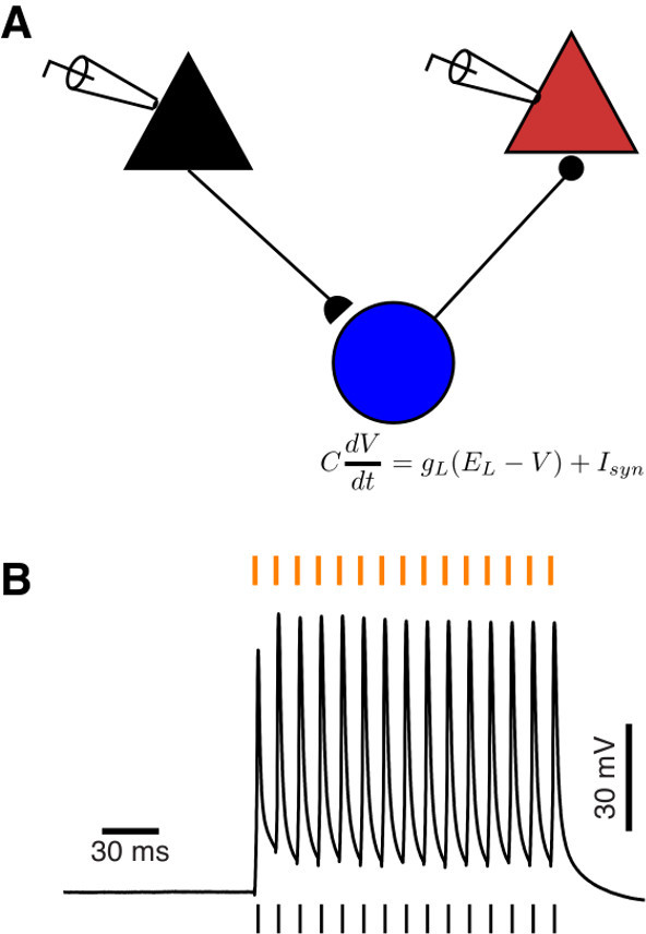
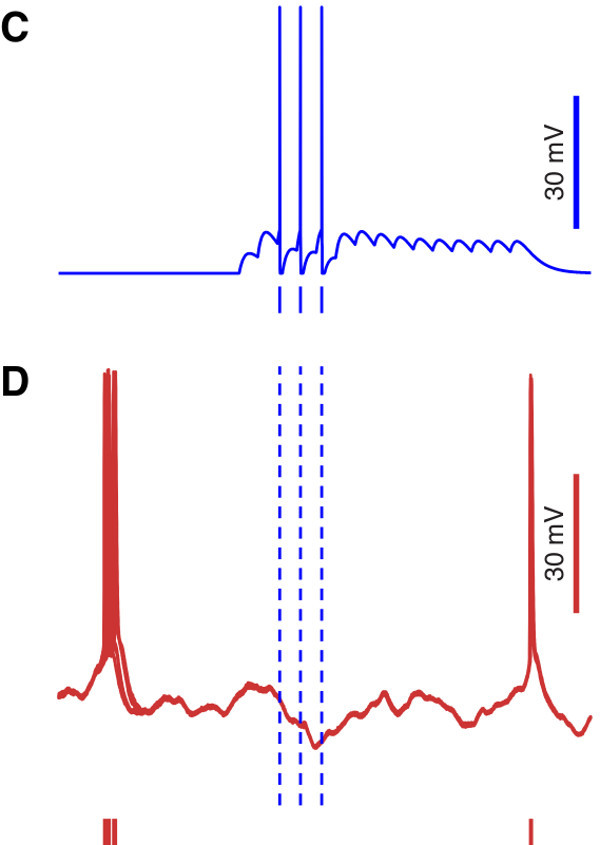
Figure 3. Simulation of disynaptic inhibition via a simulated inhibitory interneuron. (A) Schematic of the recording setup: the black and red pyramids represent a pair of real pyramidal cells recorded simultaneously. Black and red indicate presynaptic and postsynaptic neuron, respectively. The blue circle represents a virtual GABAergic interneuron, contacted by the black pyramidal cell, that in turn inhibits the red pyramidal cell. (B) Response of the real presynaptic pyramidal neuron to a train of pulses delivered at a frequency of 90 Hz, indicated by the orange dashes above the voltage trace. The black dashes below the voltage trace indicate the times action potentials were emitted by the presynaptic cell. (C) Response of the simulated interneuron to the train of spikes emitted by the presynaptic cell. (D) Superposition of 10 voltage traces recorded from the real postsynaptic pyramidal cell in response to the activation of the simulated interneuron. The postsynaptic cell was stimulated with frozen in vivo-like background activity, to obtain reliable voltage dynamics. The red dashes below the voltage traces indicate the times at which, during successive trials, the postsynaptic neurons emitted an action potential. Note the increased precision after the activation of the interneuron, indicated by a lower spike jitter across trials.

Discussion

In this text a full protocol for the implementation of real-time, closed-loop single cell electrophysiological experiments was described, using the patch clamp technique and a recently developed software toolbox called LCG. To optimize the quality of the recordings it is crucial that the recording setup be properly grounded, shielded and vibration free: this ensures stable and lasting whole-cell access to the cell, which, together with the possibility of automating entire sections of the stimulation protocols, allows for maximization of the throughput of the experiment.

Two cases in which LCG can be applied have been presented, namely the characterization of a cell in terms of its electrophysiological properties (Figure 1), including the fast computation of a neuron’s active input-output relationship, and the recreation of in vivo-like activity in a brain slice (Figure 2). Such applications showed how to construct distinct protocols and highlighted some of the most prominent features of LCG: its command-line interface makes it suited for scripting, which enables the automated application of a series of protocols. Additionally, as was done in Figure 1, values extracted from one protocol can be used to tailor parameters of subsequent protocols.

It is possible to monitor in real time higher order features of the response of the cell under analysis (e.g., its instantaneous firing rate, as shown in Figure 1D) and modify the stimulation accordingly, for instance by using a PID controller to compute the current required to maintain a constant or time-varying firing rate.

The implementation of conductance and dynamic clamp protocols with LCG is straightforward and only requires writing a text configuration file, a procedure that can be automated by the usage of simple scripts. LCG includes over 30 entities that can be interconnected to devise new experimental protocols. We described how to use LCG using a command line interface, however a graphical experiment launcher has been designed to facilitate starting experiments and changing parameters by letting non-experienced users combine LCG commands to create their own graphical interfaces.

Two existing toolboxes offer functionalities similar to LCG: RELACS and RTXI. The former is both a platform for performing electrophysiological experiments and for analyzing and annotating the recorded data. The main difference between LCG and existing solutions is its user interface based on a command-line. The advantages of this approach are several: first of all, a command-line interface allows automating standardized and repetitive tasks by means of possibly complex scripts and secondly, it allows embedding experimental trials into more complicated workflows implemented in high-level scripting language, such as Matlab or Python.

In summary, the modular nature of LCG allows expanding the number of available experimental protocols in two ways: the first and most straightforward one is by writing ad hoc configuration files that use the existing objects to perform novel protocols. The second one is by implementing – using C++ – new elementary objects that can be used to expand further the capabilities and features of LCG. The examples presented in this protocol concern the study of individual cells in brain slices. However, similar protocols can also be successfully employed in in vivo preparations, to record both intracellular and extracellular signals, and in ex vivo preparations such as neuronal cultures, to record, for instance, extracellular potentials through multi-electrode arrays while stimulating in closed-loop⁴.

Materials

List of materials used in this article

Name	Company	Catalog Number	Comments
Tissue slicer	Leica	VT-1000S
Pipette puller	Sutter	P-97
Pipettes	WPI	1B150F-4	1.5/0.84 mm OD/ID, with filament
Vibration isolation table	TMC	20 Series
Microscope	Leica	DMLFS	40X Immersion Objective
Manipulators	Scientifica	PatchStar
Amplifiers	Axon Instruments	MultiClamp 700B	Computer controlled
Data acquisition card	National Instruments	PCI-6229	Supported by Comedi Linux Drivers
Desktop computer	Dell	Optiplex 7010 Tower	OS: real-time Linux
Oscilloscopes	Tektronix	TDS-1002
Perfusion Pump	Gibson	MINIPULS3	Used with R4 Pump head (F117606)
Temperature controller	Multichannel Systems	TC02	PH01 Perfusion Cannula
Manometer	Testo	510	Optional
Incubator	Memmert	WB14
NaCl	Sigma	71376	ACSF
KCl	Sigma	P9541	ACSF, ICS
NaH2PO4	Sigma	S3139	ACSF
NaHCO3	Sigma	S6014	ACSF
CaCl2	Sigma	C1016	ACSF
MgCl2	Sigma	M8266	ACSF
Glucose	Sigma	G7528	ACSF
K-Gluconate	Sigma	G4500	ICS
HEPES	Sigma	H3375	ICS
Mg-ATP	Sigma	A9187	ICS
Na2-GTP	Sigma	51120	ICS
Na2-Phosphocreatine	Sigma	P7936	ICS

References

- Saleem, A. B., Ayaz, A., Jeffery, K. J., Harris, K. D., Carandini, M. Integration of visual motion and locomotion in mouse visual cortex. Nature neuroscience. 16, 1864-1869 (2013).
- Ahrens, M. B., Li, J. M., et al. Brain-wide neuronal dynamics during motor adaptation in zebrafish. Nature. 485 (7399), 471-477 (2012).
- Paz, J. T., Davidson, T. J., et al. Closed-loop optogenetic control of thalamus as a tool for interrupting seizures after cortical injury. Nature neuroscience. 16 (1), 64-70 (2013).
- Wallach, A., Eytan, D., Gal, A., Zrenner, C., Marom, S. Neuronal response clamp. Frontiers in neuroengineering. 3 (April), 3(2011).
- Linaro, D., Couto, J., Giugliano, M. Command-line cellular electrophysiology for conventional and real-time closed-loop experiments. Journal of neuroscience. 230, 5-19 (2014).
- Sharp, A., O’Neil, M., Abbott, L. F., Marder, E. Dynamic clamp: computer-generated conductances in real neurons. Journal of neurophysiology. 69 (3), 992-995 (1993).
- Robinson, H. P., Kawai, N. Injection of digitally synthesized synaptic conductance transients to measure the integrative properties of neurons. Journal of neuroscience methods. 49 (3), 157-165 (1993).
- Vervaeke, K., Hu, H., Graham, L. J., Storm, J. F. Contrasting effects of the persistent Na+ current on neuronal excitability and spike timing. Neuron. 49 (2), 257-270 (2006).
- White, J. A., Klink, R., Alonso, A., Kay, A. R. Noise from voltage-gated ion channels may influence neuronal dynamics in the entorhinal cortex. Journal of neurophysiology. 80 (1), 262-269 (1998).
- Destexhe, a, Rudolph, M., Fellous, J. M., Sejnowski, T. J. Fluctuating synaptic conductances recreate in vivo-like activity in neocortical neurons. Neuroscience. 107 (1), 13-24 (2001).
- Fellous, J. -M. Regulation of Persistent Activity by Background Inhibition in an In Vitro Model of a Cortical Microcircuit. Cerebral Cortex. 13 (11), 1232-1241 (2003).
- Gal, A., Eytan, D., Wallach, A., Sandler, M., Schiller, J., Marom, S. Dynamics of excitability over extended timescales in cultured cortical neurons. The Journal of neuroscience. the official journal of the Society for Neuroscience. 30 (48), 16332-16342 (2010).
- Wang, Y., Toledo-Rodriguez, M., et al. Anatomical, physiological and molecular properties of Martinotti cells in the somatosensory cortex of the juvenile rat. The Journal of physiology. 561 (Pt 1), 65-90 (2004).
- Wang, Y., Gupta, A., Toledo-Rodriguez, M., Wu, C. Z., Markram, H. Anatomical, physiological, molecular and circuit properties of nest basket cells in the developing somatosensory cortex). Cerebral cortex (New York, N.Y). 12 (4), 395-410 (1991).
- Brette, R., Piwkowska, Z., et al. High-resolution intracellular recordings using a real-time computational model of the electrode. Neuron. 59 (3), 379-391 (2008).
- Rutishauser, U., Kotowicz, A., Laurent, G. A method for closed-loop presentation of sensory stimuli conditional on the internal brain-state of awake animals. Journal of neuroscience. 215 (1), 139-155 (2013).
- Margrie, T., Brecht, M., Sakmann, B. In vivo, low-resistance, whole-cell recordings from neurons in the anaesthetized and awake mammalian brain. Pflugers Archiv European Journal of Physiology. 444 (4), 491-498 (2002).
- Graham, L., Schramm, A. In Vivo Dynamic-Clamp Manipulation of Extrinsic and Intrinsic Conductances: Functional Roles of Shunting Inhibition and I BK in Rat and Cat Cortex. Dynamic Clamp: From Principles to Applications. , (2008).
- Sakmann, B., Neher, E. Single-channel recording. , (1995).
- Molleman, A. Patch Clamping. , John Wile., & Sons, Ltd. Chichester, UK. (2002).
- Davie, J. T., Kole, M. H. P., et al. Dendritic patch-clamp recording. Nature Protocols. 1 (3), 1235-1247 (2006).
- Gold, R. The Axon Guide for Electrophysiolog., & Biophysics Laboratory Techniques... , (2007).
- Mainen, Z. F., Sejnowski, T. J. Reliability of spike timing in neocortical neurons. Science. 268 (5216), 1503-1506 (1995).
- Buzsáki, G. Action potential threshold of hippocampal pyramidal cells in vivo is increased by recent spiking activity. Neuroscience. 105 (1), 121-130 (2001).
- Koch, C., Segev, I. Methods in Neuronal Modeling: From Synapses to Networks. , MIT Press. Cambridge, MA, USA. (1988).
- Silberberg, G., Markram, H. Disynaptic inhibition between neocortical pyramidal cells mediated by Martinotti cells. Neuron. 53 (5), 735-746 (2007).
- Berger, T. K., Silberberg, G., Perin, R., Markram, H. Brief bursts self-inhibit and correlate the pyramidal network. PLoS biology. 8 (9), (2010).
- Tsodyks, M., Pawelzik, K., Markram, H. Neural networks with dynamic synapses. Neural computation. 10 (4), 821-835 (1998).
- Kapfer, C., Glickfeld, L. L., Atallah, B. Supralinear increase of recurrent inhibition during sparse activity in the somatosensory cortex. Nature. 10 (6), 743-753 (2007).
Reprints and Permissions