Mapping Dysfunctional Protein-Protein Interactions in Disease

Summary

Here, we present a protocol to enable the capture and identification of disease-specific protein-protein interactions from native cells and tissues using chemical probes and mass spectrometry. The resulting interaction datasets are analyzed through a dedicated web-based platform to reveal dynamic network dysfunctions and pathway alterations linked to disease.

Abstract

Protein-protein interaction (PPI) networks are dynamically remodeled in disease, yet most systems biology approaches focus on changes in protein abundance, overlooking critical interaction-level dysfunction. Here, we present a robust, chemoproteomic method-dysfunctional Protein-Protein Interactome (dfPPI)-that enables high-throughput, systematic, disease-contextual mapping of PPI network dysfunctions in cells and primary human tissue. This method integrates chemical biology probes that selectively capture epichaperome-based interactome assemblies with label-free liquid chromatography-tandem mass spectrometry (LC-MS/MS) and network-based computational analysis, to uncover the rewiring of protein networks not apparent from transcriptomic or proteomic data alone. The dfPPI platform can be applied across disease states, species, and tissues to identify actionable nodes of dysfunction and enable high-resolution, systems-level insights into disease progression. In this protocol, we demonstrate step-by-step procedures for sample preparation, chemical probe treatment, affinity enrichment, label-free LC-MS/MS analysis, and bioinformatics workflows used to generate and interpret dfPPI datasets. This article aims to promote reproducibility and accessibility of this approach, supporting its adoption by the broader systems biology and translational research communities.

Introduction

The function of cells, and by extension organisms, depends on the precise coordination of protein-protein interaction (PPI) networks^1,2. These networks are responsible for organizing and executing nearly all biological processes. While PPI networks are inherently dynamic and responsive to stress, in disease, they can become abnormally rewired, leading to maladaptive functions. Importantly, this rewiring does not necessarily involve changes in gene or protein expression; rather, it arises from altered physical interactions among proteins that are otherwise normally expressed^3,4,5. Traditional approaches in systems biology, such as transcriptomics or proteomics, fail to capture these critical interaction-level changes.

PPI mapping technologies have advanced significantly, offering insights into the organization and regulation of cellular networks^{6,7,8,9,10,11}. Commonly used approaches, including affinity purification-mass spectrometry (AP-MS), cross-linking (XL)-MS, proximity labelling, and co-fractionation, each offer specific advantages, such as high specificity, spatial resolution, or the ability to detect transient complexes^6,8,9,10,11. However, these methods often require bait proteins, genetic manipulation, or complex bioinformatics, and may struggle to capture the large-scale, disease-driven rewiring of protein networks in native biological systems^{6,7,8,9,10,11}. Most also lack scalability, making them impractical for analyzing large sample cohorts or systematically mapping interactome changes across conditions, cell types, or time points^{6,7,8,9,10,11} (Table 1).

To address this gap, we developed the dysfunctional Protein-Protein Interactome (dfPPI) platform, a chemoproteomic method that directly identifies the PPI network dysfunctions responsible for disease phenotypes¹². It leverages a key biological insight: in disease states, a subset of molecular chaperones form supramolecular scaffolds called epichaperomes^13,14,15. These structures do not act in protein folding but instead function as scaffolding interaction hubs that reorganize protein connectivity³. Crucially, the proteins sequestered into epichaperomes are not random; they are those actively involved in sustaining the disease phenotype^{16,17,18,19,20}. By capturing these epichaperome-bound proteins and their interactors, dfPPI identifies the exact network alterations driving specific disease states. Epichaperome-driven network rewiring is prevalent across diseases-majority in Alzheimer's disease cohorts and ~70% in cancer specimens^16,20-supporting dfPPI's applicability to large, disease-focused studies.

The dfPPI platform encompasses the entire workflow from sample preparation, epichaperome affinity capture, and interactome identification by MS, to downstream bioinformatics analyses such as pathway enrichment and functional protein network modeling (Figure 1). The method makes use of epichaperome-specific chemical probes immobilized on affinity matrices (PU-beads or other probes)^13,16,17 to isolate the functional interactome from cells or tissues. These probes have already been rigorously validated in multiple publications for specificity to epichaperomes and fitness for dfPPI^{16,17,18,20,21,22}. Captured complexes are subjected to MS, using both on-bead and in-gel digestion workflows, followed by label-free LC-MS/MS. The resulting data can then be analyzed through a dedicated bioinformatics pipeline that defines interaction-level dysfunction and links it to biological processes and phenotypes. Because epichaperomes scaffold context-specific interactomes^17,18,20, dfPPI reveals how protein networks are remodeled in a particular disease, cell type, or stage, making it a powerful systems biology tool for precision phenotyping.

The method is highly scalable and has been applied to hundreds of clinical and experimental samples, including post-mortem human tissue and cultured cells, across diverse diseases such as cancer and neurodegeneration^{16,17,18,19,20,22,23}. By uncovering the PPI changes that define a pathological state, dfPPI enables both mechanistic insight and the discovery of actionable therapeutic targets^{16,17,18,19,20,22,23}.

In this protocol, we describe in detail the experimental components of the dfPPI platform, from affinity capture of epichaperome-bound interactomes to sample preparation for LC-MS/MS to interactome identification via MS. The computational analysis pipeline-that is, what is done with the list of proteins identified by MS to define differential interactions and functional consequences-is not covered here due to space limitations. However, it is freely accessible and extensively documented via the dfPPI Shiny App at https://epichaperomics.mskcc.org (updated to https://dfppi.mskcc.org) and through the Chiosis Lab website at https://www.chiosislab.com/resources. In addition to these portals, the complete bioinformatics pipeline and accompanying scripts are included in several publications applying dfPPI to cancer^16,17,19 and Alzheimer's disease^18,20.

Protocol

The protocol follows the guidelines of our institution's human research ethics committee and animal care and use committee. Equipment and reagents used in the study are listed in the Table of Materials.

1. Sample preparation for affinity capture

1. Protein extraction from tissue
   NOTE: This protocol has been optimized for post-mortem brain tissue samples.
   1. Prepare a protein extraction buffer containing 20 mM Tris (pH 7.5), 20 mM KCl, 5 mM MgCl₂, and 0.01% NP-40 (native lysis buffer). Add protease and phosphatase inhibitors immediately before use. Keep the buffer on ice.
   2. Place the frozen tissue (target volume approximately 50 mm³) into a micro tissue homogenizer tube, which consists of a specialized 1.5 mL microcentrifuge tube fitted with a pestle. Add 500-700 µL of native lysis buffer, adjusting the volume based on tissue compactness and ease of homogenization. Homogenize the sample on ice by gently moving the pestle up and down and against the abrasive walls of the homogenizer tube until a homogeneous suspension is formed.
      NOTE: Perform all steps on ice to maintain protein assemblies in their native configuration and to avoid protein degradation.
   3. Incubate lysates at 4 °C for 30 min by placing the vial on a rotation unit. Gently mix the samples during incubation using rotation.
   4. Centrifuge the samples at 13,000 × g for 10 min at 4 °C using a benchtop centrifuge to remove debris.
   5. Collect the supernatants and transfer them into clear 1.5 mL microcentrifuge tubes. Avoid disturbing the pellet during transfer.
   6. Determine total protein concentration in the supernatant using the bicinchoninic acid (BCA) assay kit according to the manufacturer's instructions.
      NOTE: Protein lysates can be stored at -80 °C until use. Avoid repeated freeze-thaw cycles. Refer to a previous publication²⁴ for the impact of repeated freeze-thaw cycles and storage temperature on the integrity of protein assemblies.
2. Sample normalization
   NOTE: HSP90α and HSP90β are core components of the epichaperome and are the direct binding partners of the chemical probe used for interactome capture^13,21,23. Normalizing samples based on HSP90α (or HSP90β) ensures that the amount of probe-targetable epichaperome is matched across samples, which is essential for accurate comparison of the captured interactomes. Samples can be normalized based on HSP90 levels determined by Western blot, but other methods may also be used. If HSP90 levels are comparable across samples, skip this section and proceed to step 1.3. Use of HSP90α/β blotting here is for input normalization only and should not be interpreted as an epichaperome abundance measure.
   1. Prepare 2× Laemmli sample buffer consisting of 4% sodium dodecyl sulfate (SDS), 20% glycerol, 10% 2-mercaptoethanol, 0.02% bromophenol blue, and 0.125 M Tris-HCl, pH ~6.8.
      CAUTION: 2-mercaptoethanol is toxic and volatile and should be handled in a fume hood.
   2. Combine 5 µg of the total brain protein extract (from step 1.1) 1:1 (v/v) with 2× Laemmli sample buffer in a 1.5 mL clear microcentrifuge tube.
   3. Heat the samples at 95 °C for 3-5 min in a heating unit to denature proteins before loading onto sodium dodecyl-sulfate polyacrylamide gel electrophoresis (SDS-PAGE).
   4. Load the samples onto precast 8% Tris-Glycine protein gels. Alternatively, use hand-cast gels.
   5. Load 5 µL of pre-stained protein standard onto each gel, for example, into the first well, to determine protein molecular weight.
   6. Run the gels in 1× TGS (Tris-Glycine-SDS) running buffer at RT. Typical run time is 1.5-2 h at 100 V.
   7. Prepare a transfer buffer containing 25 mM Tris, 192 mM glycine, and 20% methanol.
      CAUTION: Methanol is flammable and should be handled per safety guidelines.
   8. Transfer the proteins onto a nitrocellulose membrane in transfer buffer at 4 °C for 60 min at constant voltage (100 V).
   9. Prepare a membrane washing solution (1× TBS-0.1% Tween-20) and blocking solution (5% milk in 1× TBS-0.1% Tween-20). This protocol uses powdered non-fat dry milk from a commercial source.
   10. Place the membrane in blocking solution for 1 h at room temperature (RT) with gentle agitation on a platform rocker. Use 10 mL of blocking solution per mini gel.
   11. Remove the blocking solution and incubate the membrane with anti-HSP90α antibody (1:6,000 dilution in 10 mL blocking solution) overnight at 4 °C on a platform rocker.
   12. Remove the antibody solution and wash the membrane three times for 5 min each with 10 mL of washing solution.
   13. Add the HRP-conjugated goat anti-rabbit secondary antibody (1:5,000 dilution in 10 mL 1× TBS-0.1% Tween-20) and incubate for 1 h at RT on a platform rocker.
   14. Remove the secondary antibody and wash the membrane four times with washing solution (same volume and timing as above).
   15. Detect the HSP90α-specific chemiluminescent signal using an enhanced chemiluminescence (ECL) kit according to the manufacturer's instructions. Use a chemiluminescence imaging system or autoradiographic film.
   16. Quantify HSP90α levels in the samples based on signal intensity and calculate a normalization factor for downstream pull-down.
       ​NOTE: The intensity of the HSP90 signal reflects the amount of probe-targetable epichaperome in each sample. By comparing signal intensity between samples and normalizing to a reference sample run on every gel, input volumes for interactome capture can be adjusted accordingly. Quantification can be performed using densitometry software. Always include an aliquot of a reference sample on each gel to allow for normalization across blots.
3. PU-bead preparation
   NOTE: PU-beads and control beads can be synthesized in-house as previously reported^21,25 or requested from the Chiosis laboratory upon execution of a material transfer agreement (MTA). They should be stored at -20 °C in isopropanol.
   1. Take an aliquot of polyurethane (PU)-beads or control beads directly from the isopropanol stock. Include approximately 30% excess to account for bead loss during washing and handling.
   2. Remove the storage solvent: let beads settle, then aspirate the isopropanol. Add native lysis buffer (1 mL for a 1.5 mL tube; 5 mL for a 15 mL conical) and fully resuspend by gentle pipetting or inversion.
   3. Wash and equilibrate three times: for each wash, vortex to resuspend, centrifuge (1.5 mL tube: 10,000 × g, 1 min; 15 mL conical: 3,000 × g, 5 min), then aspirate the supernatant with a vacuum line fitted with a pipette tip, taking care not to disturb the pellet.
   4. Add native lysis buffer to the washed beads at a 1:1 volume ratio (beads:buffer) to generate a uniform working bead slurry.
   5. Aliquot 40 µL of PU-bead (or control bead) slurry (e.g., 1:1 v/v beads:buffer) per sample into 1.5 mL microcentrifuge tubes. Use a pipette tip with the end cut off to allow for easy bead dispensing.
      NOTE: PU-beads are light sensitive. Use dark or foil-wrapped 1.5 mL tubes during pull-down steps. Due to their hydrophobic surface coating with the small molecule epichaperome binder, PU-beads tend to clump and adhere to plastic surfaces. Pipette gently and mix thoroughly to ensure uniform resuspension. It is critical to dispense equal volumes of bead slurry into each sample to avoid variability in protein capture, which can lead to inconsistent or non-reproducible results.
   6. Wash the beads three times with native lysis buffer by adding 1 mL of buffer to each tube, vortexing, centrifuging at 10,000 × g for 1 min, and discarding the supernatant by aspiration. Ensure beads are fully resuspended between each wash.
      NOTE: When aspirating, avoid touching the beads. Press the pipette tip gently against the wall of the tube while removing the liquid.
   7. After the final wash, remove most of the liquid from the tubes, taking care not to disturb the bead pellet.
      NOTE: Washed beads can be stored at 4 °C for a few days. Typically, the beads are used within 1-2 days after preparation.
4. Interactome pull-down
   NOTE: The first step of the pull-down is a pre-clearing step using control beads, which are conjugated to an inert small molecule that does not bind epichaperomes¹⁶. This step removes non-specifically interacting proteins, aggregates, and insoluble debris from the lysate, thereby improving the specificity of the subsequent PU-bead pull-down. Pre-clearing reduces background binding and enhances detection of specific epichaperome-associated proteins.
   ​The interactome recovered by this protocol is analyzed by MS, which is highly sensitive to experimental contaminants. To ensure accurate protein identification and preserve data quality, always use freshly prepared buffers and reagents, minimize exposure to dust and keratin, and wear clean, powder-free gloves when handling samples, consumables, or equipment. Use MS-dedicated glassware/consumables for all pull-down and in-gel digestion steps, and keep any items used for Western blotting physically separate. If reusing glassware, decontaminate by rinsing sequentially with 100% methanol, ultrapure water, 80% acetic acid, ultrapure water, then air-dry. Do not use detergents; even trace residues can foul LC columns and ion sources.
   1. Add the normalized protein extracts (as per step 1.2, calculated based on HSP90 blot intensity) to individual 1.5 mL microcentrifuge tubes containing 40 µL of the control beads slurry (i.e., 20 µL beads + 20 µL buffer), and adjust the final volume to 250 µL by adding the appropriate volume of native lysis buffer.
      NOTE: To determine sample-specific input volumes, use the formula A1 = (60 / C1) × X1, where A1 is the volume of normalized total protein to add (µL), C1 is the measured protein concentration (µg/µL), and X1 is the normalization factor derived from HSP90 blotting (as described in step 1.2). The volume of additional buffer to add is calculated as 250 µL minus A1. If normalization is not needed, use 250 µg total protein in 250 µL.
   2. Incubate the samples at 4 °C for 30 min with rotation on an end-over-end rotator (10-15 rpm).
   3. Centrifuge the tubes at 10,000 × g for 1 min at 4 °C to pellet the control beads along with aggregated or insoluble protein.
   4. Carefully collect the supernatant from the control beads using a 1 mL pipette and transfer it to 1.5 mL tubes containing 40 µL of the washed PU-beads slurry.
   5. Incubate the samples at 4 °C for 3 h with rotation on an end-over-end rotator (10-15 rpm).
   6. Centrifuge each tube at 10,000 × g for 1 min, aspirate the supernatant, and wash the beads four times with 1 mL of native lysis buffer. For each wash: vortex, centrifuge, and aspirate, using the parameters described in step 1.3.
      NOTE: At this stage, the samples can be processed for LC-MS/MS using one of two workflows:(1) SDS-PAGE followed by in-gel digestion, or (2) on-bead digestion of the captured proteins.
      For the in-gel digestion workflow, continue with the protocol as written. For on-bead digestion, wash the beads two additional times with cold PBS and proceed immediately to Section 3. Do not freeze the beads if proceeding with on-bead digestion; samples must be processed fresh on the same day. Freezing bead-bound protein complexes can impair digestion efficiency by promoting aggregation or loss of protein solubility, leading to lower peptide recovery and increased variability. Based on MS core recommendations, samples should be processed fresh on the same day to ensure consistent on-bead digestion.
5. Sample preparation for in-gel digestion
   1. Add 25 µL of 2× Laemmli sample buffer to the bead samples prepared in step 1.4.6, which are contained in 1.5 mL microcentrifuge tubes.
      NOTE: The samples at this point can be stored at -80 °C for up to 24 h. Always load the entire sample volume to the SDS-PAGE gel for in-gel digestion to maximize proteome coverage and ensure full representation of the interactome. Partial loading is not recommended. If the sample volume is limited and partial loading is unavoidable, the remaining material should be stored in aliquots to minimize freeze-thaw cycles and preserve interactome integrity.
   2. Heat each sample at 95 °C for 3 min (with the added 2× Laemmli sample buffer, as above) to denature the protein complexes and elute them from the beads before loading onto SDS-PAGE. The SDS and reducing agents in the buffer disrupt PPIs and release proteins from the matrix.
   3. Centrifuge each tube at 10,000 × g for 1 min at RT.
   4. Load each supernatant onto 4-20% precast gradient SDS-PAGE gels.
   5. Run the gels in 1× TGS running buffer at RT and stop the run halfway through (~3.5-4 cm into the gel at 100 V, typically 30-60 min runtime).
   6. Remove the gel from the electrophoresis unit and proceed to stain with Coomassie brilliant blue according to the manufacturer's instructions.
      NOTE: The stained gel, immersed in 5-7 mL of ultrapure water in a plastic container, can be transported to the MS facility for protein identification. If not immediately processed, store at 4 °C in ultrapure water for up to 1-2 weeks. Two alternative proteomic workflows were used depending on the core facility that performed the work and experimental goals: Section 2 describes in-gel digestion followed by data-independent acquisition(DIA)-MS analysis using quadrupole orbitrap mass spectrometer; Section 3 details an on-bead digestion protocol optimized for trapped ion mobility spectrometry with parallel accumulation-serial fragmentation (diaPASEF)²⁶. Steps may be cross-referenced where appropriate.

2. Protein Identification by LC-MS/MS with in-gel protein digestion

1. In-gel reduction and alkylation of cysteinylated proteins
   1. Excise the stained region of each Coomassie-stained gel lane and cut it into approximately five equally sized gel slices. Destain each slice by incubating it three times in 500 µL of 50% (v/v) methanol for 1 min at 37 °C with agitation at 700 rpm on a temperature-controlled microtube shaker.
      NOTE: Each gel slice should be no larger than ~1 cm × 0.5 cm × 1 cm to ensure efficient diffusion of reagents in subsequent steps as well as efficient in-gel trypsin digestion overnight. Excise the gel region corresponding to heavily stained proteins-such as HSP90 and HSC70, which represent direct binders of the chemical probe and core components of the epichaperome^15,16,23-separately from the rest of the gel. Their high abundance may otherwise interfere with the detection and quantification of lower-abundance interactors during LC-MS/MS analysis.
   2. Incubate each gel slice in 500 µL of 5 mM ammonium bicarbonate (ABC) prepared in 30% acetonitrile (ACN) at 37 °C with shaking at 700 rpm on a temperature-controlled microtube shaker for 15 min to remove residual stain. Repeat the incubation until the gel slice is completely destained.
      NOTE: Any remaining visible protein stain can interfere with peptide binding to the C18 matrix during the peptide cleanup step, reducing recovery and downstream MS sensitivity.
   3. Remove and discard the ABC/ACN solution using a fine-tip pipette, taking care not to lose the gel pieces (i.e., do not aspirate the gel pieces along with the liquid). Then add 500 µL of 100% ACN to each tube, ensuring the gel pieces are fully submerged. Incubate at RT on an orbital shaker at 700 rpm for 10 min, or until the gel pieces become translucent, shrink in size, and take on the appearance of white paper.
      CAUTION: ACN is flammable and should be handled in a fume hood.
   4. Remove and discard the ACN from each tube using a fine-tip pipette, taking care not to aspirate gel pieces. Briefly centrifuge at 1,000 × g for 10 s to collect residual liquid, and carefully aspirate remaining droplets with a fine-tip pipette. Place the open tubes in a vacuum centrifuge at RT for 10-15 min, or until the gel slices are dry and rigid.
      NOTE: Do not overdry. Check periodically to avoid cracking or over-shrinkage of gel pieces. Once dried, store the gel pieces at 4 °C in a sealed, low-binding tube or microcentrifuge tube until digestion; gel-bound and purified proteins are stable up to several days when kept at 4 °C.
   5. Reduction: Add ~100 µL of 10 mM Dithiothreitol (DTT) (prepared fresh from 500 mM stock in 50 mM ammonium bicarbonate) to each sample tube, ensuring the gel pieces are fully submerged. Incubate at 56 °C for 45 min with agitation at 700 rpm on a temperature-controlled microtube shaker.
      CAUTION: DTT is a skin and respiratory irritant. Handle inside a chemical fume hood and wear gloves.
      NOTE: Ensure tubes are tightly closed during incubation to avoid evaporation and maintain DTT concentration.
   6. Alkylation: Remove the DTT solution from each tube using a fine-tip pipette, taking care not to disturb the gel pieces. Immediately add ~100 µL of 55 mM iodoacetamide (IAA) in 50 mM ABC to fully cover the gel slices. Incubate at RT with agitation at 700 rpm for 30 min in the dark.
      CAUTION: IAA is toxic and light sensitive. Perform all handling in a fume hood while wearing gloves.
      NOTE: Ensure complete removal of DTT before adding IAA to avoid quenching of the alkylation reaction. Wrap tubes in aluminum foil or use light-blocking containers during incubation to minimize IAA degradation.
   7. Centrifuge the tubes briefly at 1,000 × g for 5 s at RT to collect residual liquid at the bottom. Carefully remove the supernatant using a fine-bore pipette tip (e.g., P10 tip) to avoid disturbing the gel pieces. Tilt the tube slightly and aspirate from the edge to minimize the risk of aspirating gel fragments.
   8. Equilibrate: Cover the gel pieces with 500 µL of 50 mM ABC in 30% ACN. Incubate at RT for 10 min, agitating at 700 rpm on a heated orbital shaker. This step helps remove excess alkylation reagent and equilibrates the gel prior to dehydration.
   9. Remove solution: Briefly spin at 1,000 × g for 5 s and discard the supernatant using a fine-tip pipette, as described above.
   10. Dehydrate again: Repeat steps 2.1.3 and 2.1.4 to re-dehydrate the gel pieces using 100% ACN followed by vacuum centrifugation until dry. This step ensures optimal peptide recovery during enzymatic digestion.
2. In-gel proteolysis and peptide cleanup
   1. Digest the dried gel samples by adding MS-grade trypsin at a final concentration of 5 ng/µL in 50 mM ABC to fully rehydrate the gel pieces (typically 50-100 µL total volume, or enough to cover gel slices). Incubate overnight at 37 °C in 1.5 mL microcentrifuge tubes, ensuring tubes are sealed tightly to prevent evaporation. Agitate gently if possible (e.g., 300 rpm on a temperature-controlled microtube shaker).
   2. Acidify the sample following overnight digestion by adding 10% formic acid (FA) dropwise to achieve a final concentration of 1% (v/v) (e.g., add 1 µL of 10% FA to 100 µL digest). Mix gently, then sonicate the tubes for 10 min in a RT water bath sonicator to enhance peptide extraction.
   3. Carefully remove the peptide-containing supernatant using a fine-tip pipette (e.g., P10 narrow-bore tip), taking care not to disturb the gel matrix or aspirate gel fragments. Transfer the collected supernatant into a low-bind 500 µL tube and place it on ice.
   4. Add 5% FA/50% ACN (v/v) solution to each tube (typically ~50-100 µL, or enough to fully cover the gel pieces), and agitate gently at RT (e.g., on a shaker at 70 rpm for 10-15 min) to extract residual peptides. Carefully collect the supernatant and combine it with the original peptide solution from step 2.2.3.
   5. Concentrate the combined peptide extract using vacuum centrifugation at RT (e.g., 1,000 × g for ~30 min) until only a small droplet remains. Do not allow the sample to dry completely, as this may cause peptide loss due to adherence to tube walls. Use the partially dried extract either immediately for desalting or store at -20 °C in a sealed, low-bind tube.
   6. Desalt the peptides using hand-packed small-scale C18-packed pipette tips (i.e., StageTips) prepared with two stacked C18 extraction discs inserted into a 200 µL pipette tip, as described previously²⁷, with the following modifications:
   7. Activate the C18 discs by adding 40 µL of methanol. Centrifuge the pipette tip containing the discs (inserted into an empty 200 µL pipette tip and placed inside a 500 µL tube) using a benchtop centrifuge at 1,500 × g for 3 min.
      ​NOTE: At all steps, do not allow the C18 discs to dry. Drying will interfere with peptide binding and elution. The outer 200 µL pipette tip (sleeve) holding the hand-packed small-scale C18 packed pipette tip may need to be shortened by cutting ~ 1 cm from the end to ensure the two-tip-in-tube assembly fits properly in the centrifuge.
   8. Equilibrate the discs by adding 0.1% FA and centrifuging as above.
   9. Apply the peptide solution, reconstituted in 20 µL of 0.1% FA, directly onto the top of the stacked discs.
   10. Centrifuge at 1,500 × g for 5 min to facilitate peptide binding to the C18 discs.
   11. Wash the bound peptides by passing 40 µL of 0.1% FA through the column.
   12. Elute peptides with 40 µL of 70% ACN containing 0.1% FA. Store the eluted peptides in low-binding tubes at -80 °C until LC-MS/MS analysis. Avoid repeated freeze-thaw cycles.
3. Nano-LC coupled to MS analysis using DIA
   1. Concentrate the desalted peptide eluate using vacuum centrifugation (e.g., 20-30 min at RT, 1,000 × g), leaving a small droplet. Reconstitute the peptides in 10 µL of 0.1% FA in LC-MS-grade water by pipetting up and down gently and briefly vortexing. Spin down briefly to collect liquid at the bottom of the tube before proceeding.
   2. Analyze 4 µL aliquots of the reconstituted peptide sample by nano-LC-MS/MS. Separate the peptides on a self-packed reverse-phase column (75 µm ID × 2 cm, C18 resin, 3 µm particle size) maintained at 50 °C. Prepare the column using a pressure bomb²⁸ by packing a slurry of C18 resin (in methanol, 1:3 v/v) into a fused silica capillary with an integrated 10 µm spray tip (360 µm OD × 75 µm ID × 10 µm tip). Interface the column via nanospray ionization to a high-resolution hybrid mass spectrometer (quadrupole-Orbitrap-type) supporting DIA workflows.
      ​NOTE: A 20 cm column length is recommended as it provides optimal separation for peptide mixtures generated from SDS-PAGE gel slices.
   3. Maintain the analytical column at 50 °C using a column oven or heating block to ensure consistent peptide retention and separation. Ensure stable temperature control throughout the run, as fluctuations can affect reproducibility.
   4. Elute peptides using a linear gradient of 3-40% ACN in 0.1% FA over 110 min, at a flow rate of 250 nL/min. This gradient provides effective peptide separation prior to MS detection. The total analysis time, including column equilibration, is 120 min.
   5. Acquire data in DIA mode using a high-resolution MS, as described previously²⁹.
      1. Set full MS1 survey scans to be acquired in profile mode at a resolution of 120,000 (at m/z 200), over a scan range of 300-1650 m/z. Follow each MS1 scan with MS2 fragmentation of 30 sequential precursor windows (364-1370 Th) using a sliding isolation window scheme.
      2. Perform fragmentation using stepped normalized collision energies of 25.5, 27.0, and 30.0. The default maximum precursor charge state is 4. Set the fixed first mass in MS/MS scans to 200 Da, and acquire MS2 spectra at a resolution of 30,000.
      3. Use an automatic injection time setting for MS2 and a 60 ms maximum injection time for MS1. For both MS1 and MS2 scans, set the ion target (AGC) to 3e6.
4. Relative quantification of affinity-captured interactomes
   NOTE: To quantify proteins identified in DIA-MS analyses of affinity-captured epichaperome interactomes, use a software platform that supports DIA workflows and provides reliable quantification based on peptide intensity or spectral counts. This protocol used MaxQuant (e.g., version 2.5.1.0) and its MaxDIA workflow^20,29 for peptide/protein identification and label-free intensity-based quantification. Searches used a reversed-sequence decoy strategy with 1% FDR at PSM/peptide and protein levels; "Reverse" and "Potential contaminant" entries were filtered before bioinformatics. No spike-ins were used; instrument readiness was verified with 250 ng of HeLa digest (and intermittent 10 fmol 6-protein mix) meeting internal ID and RT-stability criteria.
   1. Analyze raw DIA-MS data with consistent parameters across all samples. Include up to two missed cleavages and set modifications as follows: fixed, carbamidomethylation of cysteine; variable, oxidation of methionine, and acetylation of the protein N-terminus.
   2. Use an in silico-predicted spectral library based on the UniProt human protein database (e.g., ~20,000 entries), ensuring that decoy and contaminant sequences are included for accurate false discovery rate (FDR) estimation. Specify tryptic digestion unless an alternative enzyme was used. A validated human spectral library (based on the 06/18/2020 UniProt release, 20,956 entries) is available from the Max Planck Institute of Biochemistry repository³⁰.
      NOTE: As an alternative to this workflow with predicted libraries, step 3.4 illustrates library-free processing, which produced comparable identification and quantification on these datasets.
   3. Quantify protein abundances using intensity values (not label-free quantification [LFQ] intensities), as these are more appropriate for downstream PPI network analyses. Ensure that LFQ is deselected to avoid normalization artifacts, which can distort affinity-enrichment data. Instead, use raw intensity values derived from peptide spectral matches, which reflect interaction strength rather than global protein expression. Apply appropriate filtering criteria (e.g., minimum one unique peptide per protein group) to improve the reliability of protein identification and quantification. Export the resulting protein intensity table for subsequent statistical and network-based analyses.
      NOTE: Unlike standard proteomic workflows, where LFQ values help normalize for protein loading across whole lysates, here proteins are enriched through affinity capture of epichaperomes. This enrichment step introduces biological variance that LFQ normalization may obscure. Therefore, raw intensity values are preferred, as they better reflect the differential protein-epichaperome interactions across conditions and preserve signal needed for downstream network-level (e.g., dfPPI) analysis. In prior studies using Mascot-based searches^16,18, MS/MS spectral count values were also used in place of intensities. In affinity capture workflows such as this, spectral counts reflect interaction frequency and are well-suited for identifying differentially interacting proteins across conditions. Unlike LFQ values, MS/MS counts do not assume global normalization across the proteome, preserving biologically meaningful variance from the epichaperome enrichment step.

3. Protein Identification by LC-MS/MS with on-bead protein digestion

1. On-bead digestion
   NOTE: To ensure optimal protein recovery and minimize sample loss during on-bead protein digestion for MS analysis, it is essential to use low-protein binding microcentrifuge tubes. These tubes are designed to reduce protein absorption to the tube walls, thereby enhancing sample recovery. All reagents used in this section should be freshly prepared using LC-MS-grade water and chemicals. If submitting samples to a proteomics core, check local policies, as some facilities may require that all buffers be filter sterilized before use.
   1. Remove any residual PBS that may remain in the tube from step 1.4.6. Resuspend the beads in 80 µL of 2 M urea, freshly prepared in 50 mM ABC, pH 8.5. Ensure complete mixing by pipetting or brief vortexing.
      NOTE: Adjust the volume proportionally based on bead quantity and type. This protocol is optimized for 40 µL of PU-beads slurry.
   2. Add DTT to achieve a final concentration of 1 mM.
      NOTE: Prepare a fresh 10 mM DTT solution from a 1 M DTT stock solution in LC-MS grade water immediately before use, as DTT is prone to oxidation in solution. Add the required volume directly to the sample and mix gently by pipetting.
   3. Cap the tube and incubate at 37 °C for 30 min with shaking at 1,100 rpm on a heated orbital shaker. Seal lids tightly to minimize evaporation.
   4. Add IAA to reach a final concentration of 3.67 mM. Incubate in the dark at RT for 45 min with shaking at 1,100 rpm.
      NOTE: Prepare a fresh 10 mM IAA stock in LC-MS grade water immediately before use. Add the required volume to the sample and mix gently by pipetting.
   5. Add additional DTT to quench unreacted IAA, achieving a final concentration of 3.67 mM. Mix gently by pipetting.
      NOTE: Quenching unreacted IAA prevents over-alkylation, which can compromise protease activity and digestion efficiency. Prepare DTT fresh and calculate the volume based on the current sample volume to achieve the target concentration.
   6. Add 750 ng of 0.5 mg/mL of MS-grade Lys-C protease to the sample. Incubate at 37 °C for 1 h with shaking at 1,150 rpm.
      NOTE: Prepare Lys-C by dissolving in LC-MS grade water. Store enzyme aliquots at -80 °C and avoid multiple freeze-thaws.
   7. Add 750 ng of 0.5 mg/mL of sequencing-grade trypsin freshly prepared. Incubate overnight at 37 °C with shaking at 1,150 rpm. Incubate no longer than 16-18 h to prevent overdigestion and peptide degradation.
   8. The following day, centrifuge the sample at 1,000-5,000 × g for 1-5 min at RT and transfer the supernatant by pipetting to a fresh 1.5 mL microcentrifuge tube. Discard the beads.
   9. Adjust the pH of the digest to below 3 by adding 50% trifluoroacetic acid (TFA) dropwise. Verify the pH using pH indicator strips.
      NOTE: The typical pH range should be ~2.5-3.0, and the samples should be acidified before desalting.
      CAUTION: TFA is corrosive and volatile. Add in a fume hood and wear proper personal protective equipment (PPE).
2. Peptide desalting
   NOTE: For peptide desalting and cleanup, use small-scale C18-packed pipette tips (i.e., StageTips)³¹. Prepare C18 StageTips by packing three layers of C18 material (e.g., C18 solid-phase extraction disks) into a 200 µL pipette tip. Pre-made, commercially available C18 spin columns can also be used. Follow the manufacturer's protocol for conditioning, sample loading, and peptide elution. Performance (e.g., retention efficiency, recovery yield) may vary between homemade vs. commercial devices. Small-scale C18-packed pipette tips should be packed tightly to avoid bypass flow.
   1. Condition the small-scale C18-packed pipette tips sequentially with: (1) 100 µL methanol. Centrifuge at 400 × g and discard the flowthrough; (2) 100 µL of 70% ACN/0.1% TFA. Centrifuge at 400 × g and discard the flowthrough; (3) 100 µL of 0.1% TFA. Centrifuge at 400 × g and discard the flowthrough. Repeat this step twice.
      NOTE: Conditioning ensures full wetting of the hydrophobic C18 resin. For pre-made, commercially available C18 spin columns, vacuum manifolds can also be used. Users should refer to the manufacturer's instructions for specific handling recommendations.
   2. Load the acidified peptide digest onto the conditioned small-scale C18-packed pipette tips by slowly pipetting the sample directly into the tip. Centrifuge at 300 × g to allow the digest to pass through the resin, and discard the flowthrough. If the sample volume exceeds capacity, load in multiple rounds.
      NOTE: Pipette the digest directly onto the packed resin bed, avoiding air bubbles. If using low-retention tips, touch the inner wall of the small-scale C18-packed pipette tips to release the liquid slowly and evenly.
   3. Pipette 100 µL of 0.1% FA directly into the small-scale C18-packed pipette tip, ensuring the solution fully saturates the C18 material. Centrifuge at 400 × g and discard the flowthrough. Repeat this step twice to remove salts and interfering substances.
      NOTE: Make sure the liquid flows fully through the C18 material before each spin. Avoid trapping air bubbles by dispensing the wash solution slowly down the wall of the pipette tip.
   4. Elute the bound peptides by pipetting 50 µL of 70% ACN/0.1% FA into the small-scale C18-packed pipette tip. Centrifuge at 300 × g and collect the eluate in a clean low-bind microcentrifuge tube. Repeat this step twice to ensure complete elution.
      NOTE: Multiple rounds of centrifugation may be required to fully recover the eluate. If residual liquid remains trapped at the tip base, gently tap the small-scale C18-packed pipette tip or perform brief additional spins to collect the remaining volume. Combine eluates and check the final volume before proceeding.
   5. Freeze and dry the eluted peptides using a vacuum concentrator until dry. Ensure the lid is loosely placed to allow venting, but avoid splashing.
   6. Reconstitute the dried peptides by adding 12 µL of 0.1% FA in LC-MS-grade water directly to the bottom of the tube. Gently vortex and sonicate the tubes to fully dissolve the peptides.
      ​NOTE: Ensure that the entire pellet or dried film is fully reconstituted. Pipette-based dissolution risks peptide loss due to adherence to tip surfaces.
   7. Sonicate the reconstituted peptides for 5 min in a bath sonicator filled with cool water to ensure complete dissolution and prevent overheating.
   8. Centrifuge the peptides at 20,000 × g at 4 °C for 10 min. Transfer the peptide supernatant into an appropriate autosampler vial for loading onto the LC-MS system. Use low-volume, high-quality, gas chromatography (GC)-tested polypropylene vials with bonded silicone/polytetrafluoroethylene (PTFE) septum caps to minimize sample loss. Label vials clearly with sample ID and injection order.
   9. Estimate peptide concentration using a spectrophotometer at 280 nm. Note this is approximate and can be affected by aromatic residue content or contaminants. Alternatively, use colorimetric peptide assays for more accurate quantification.
3. LC and MS parameters
   ​NOTE: The following LC and MS parameters are optimized for the nano-LC system coupled with the mass spectrometer used in the current protocol. For other nano-LC systems and mass spectrometers, parameters should be adjusted accordingly.
   1. Prepare the mobile phases weekly to ensure LC-MS compatibility and minimize contamination: (1) Mobile Phase A: Add 1 mL of LC-MS grade FA to 1 L of LC-MS grade water, and (2) Mobile Phase B: Add 1 mL of LC-MS grade FA to 1 L of LC-MS grade ACN.
      NOTE: Use only LC-MS grade solvents and acid. Prepare both phases in clean glass bottles and degas if required by the LC system. Discard unused phases on a weekly basis to avoid microbial growth or degradation.
   2. Install a 25 cm long, 75 µm inner diameter fused-silica capillary column packed with 1.7 µm C18 reversed-phase particles.
      NOTE: Handle columns with care to avoid introducing air bubbles or damaging the packing material. Follow the manufacturer's instructions for installation and column equilibration.
   3. Condition the column by gradually increasing the flow rate from 50 nL/min to 300 nL/min using 3% Mobile Phase B.
      ​NOTE: This step ensures that the stationary phase is properly wetted and equilibrated before sample injection. Monitor column pressure during flow rate ramping. Sudden pressure spikes may indicate air bubbles or column blockage. Equilibration can be considered complete when baseline pressure stabilizes.
   4. Maintain the column temperature at 50 °C to ensure optimal chromatographic performance.
   5. Inject 100 ng of a HeLa cell tryptic digest as a quality control (QC) standard to assess system performance.
      NOTE: This QC injection serves as a benchmark to evaluate LC retention time consistency, MS sensitivity, and proteome coverage across runs. Compare protein identification counts, retention time reproducibility, and signal intensity to a reference QC dataset to confirm system readiness before analyzing experimental samples. Use commercial HeLa digest standards prepared at known concentrations for reproducibility across experiments.
   6. Employ a gradient elution from 2% to 35% mobile phase B over 90 min at a flow rate of 300 nL/min. The 90-min gradient provides high-resolution peptide separation suitable for complex proteomes. Following the gradient, hold at 95% Mobile Phase B for 7 min to wash the column.
      NOTE: Include a re-equilibration step (e.g., return to 2% B for 10-15 min) before the next injection to ensure column reproducibility across runs. Avoid abrupt gradient changes, which can impact retention time stability and peak shape.
   7. Conduct MS analysis using a mass spectrometer equipped with a nanoflow-compatible electrospray ionization source (e.g., CaptiveSpray-style).
      ​NOTE: The CaptiveSpray ion source provides stable electrospray at low nanoflow rates, enhancing ionization efficiency and sensitivity. For labs using alternative mass spectrometers adjust acquisition and ionization parameters accordingly. Ensure proper tuning and calibration before analysis to maintain accuracy and resolution. Position the spray emitter properly and monitor spray stability during the run to prevent signal dropouts.
   8. Utilize a data-independent acquisition diaPASEF method³². For users unfamiliar with diaPASEF, consult the manufacturer's technical documentation or recent protocols describing trapped ion mobility spectrometry (TIMS)-DIA workflows³³ to optimize for different sample types or gradient lengths.
      NOTE: diaPASEF combines TIMS with DIA to increase sequencing speed and sensitivity by aligning precursor and fragment ions in the mobility dimension³⁴. Ensure the TIMS device is properly calibrated and synchronized with the quadrupole to avoid misalignment of ion mobility and mass windows.
   9. Use the following instrument settings: (1) Mass range: 100 to 1700 m/z; (2) Ion mobility range: 0.60-1.60 V·s/cm²; (3) Collision energy: 20-59 eV, ramped; (4) Ramp time: 100 ms; (5) Accumulation time: 100 ms; (6) Mass range for diaPASEF: 400-1201 Da; (7) Mass window width: 26 Da with 1 Da overlap; (8) Number of mass steps per cycle: 32; (9) Cycle time: ~1.8 s
      NOTE: These settings are optimized to balance depth of coverage and scan speed. Minor adjustments (e.g., window width or number of steps) may be required depending on sample complexity, gradient length, and LC-MS system performance. Achieving identification of over 7,500 proteins for the HeLa digest indicates optimal system performance. The number of identifications may vary by instrument and should be assessed accordingly.
   10. Load 300-400 ng of peptide sample per injection to prevent overloading the analytical column. Overloading can lead to peak broadening, ion suppression, and reduced reproducibility. Confirm peptide concentration prior to injection using a spectrophotometer or colorimetric peptide assay to avoid variability across runs.
   11. Run blank injections between sample groups to avoid carryover. Use 100% mobile phase A (water with 0.1% FA) as the injection blank. This flushes residual peptides from the column and reduces contamination between runs. Monitor baseline and background ions to confirm adequate cleaning.
4. DIA data analysis
   1. Use a suitable software supporting data analysis using the directDIA workflow³⁵ and library-free processing of DIA proteomics data. Perform protein identification and quantification based on a UniProt FASTA database³⁶, with standard search parameters and default quantification settings.
      NOTE: All parameters, including enzyme specificity, modification settings, FDR thresholds, and post-analysis outputs, are detailed in the Supplementary File 1. Alternative DIA analysis platforms such as DIA-NN³⁷ may also be used if they support similar workflows and outputs.
   2. Run library-free directDIA with q-value cutoffs corresponding to 1% FDR at the precursor, peptide, and protein-group levels; exclude decoy identifications prior to downstream analysis.
      NOTE: No iRT standards were added; performance was benchmarked with HeLa digest runs against predefined identification and retention-time stability criteria.

Results

Following the successful execution of the protocol, users should obtain high-quality interaction datasets suitable for downstream dfPPI analysis. Protein identification is performed from DIA data at 1% FDR (PSM and protein levels), and quantification uses raw intensities or MS/MS spectral counts (not LFQ). Expected QC signatures include: tight clustering of technical replicates by PCA, median precursor/protein CVs of approximately 10-12%, hierarchical clustering driven by biological origin rather than replicate, and robust pathway-level enrichment on g:Profiler/Reactome.

PU-bead probe generation and activity validation prior to use

PU-beads are prepared by coupling an epichaperome-binding small-molecule analog to NHS-activated agarose, as previously described²⁵. A standard 25 mL resin pack yields ~25 mL of PU-beads stored as a 1:1 slurry in isopropanol. Aliquot into low-bind tubes and store at −20 °C, protected from light (e.g., wrap in aluminum foil). Under these conditions, a batch remains stable for ≥12 months. Before use, remove isopropanol and equilibrate beads in native binding buffer (step 1.3). Each lot is qualified at synthesis and periodically thereafter using two assays (Figure 2): (i) Biological specificity-perform matched pull-downs from an epichaperome-high lysate (e.g., MDA-MB-468) and an epichaperome-low lysate (e.g., ASPC1) under identical conditions (40 µL bead slurry with 250 µg total protein; 3 h at 4 °C; native washes), elute/denature, and immunoblot for HSP90, HSC70, and HOP. Acceptance: strong enrichment in the epichaperome-high sample with minimal signal in the low sample; band-intensity ratios comparable to a reference lot (±20-30%). (ii) Global cargo profile-run parallel captures from an epichaperome-high lysate with PU-beads versus matched inert control beads, load equal eluate volumes on SDS-PAGE, and Coomassie-stain. Acceptance: PU-beads show a rich, high-molecular-weight cargo with minimal background in the control-bead lane. A 25 mL batch supports ~600 captures at 40 µL per sample; retire a lot if the specificity or cargo profile falls outside acceptance after re-washing/re-equilibration.

Representative results of in-gel and on-bead protocols

In a pilot head-to-head comparison on epichaperome-high MDA-MB-468 cells, in-gel and on-bead workflows produced highly concordant interactomes: 4,616 of 6,333 proteins (73%) were shared at the protein-group level, with 1,275 (20%) detected only by in-gel and 442 (7%) only by on-bead. Pathway-level agreement was even higher: among 860 Reactome terms, 727 (85%) were common, with 81 (9%) unique to in-gel and 52 (6%) unique to on-bead. Median protein intensities were ~3× higher for in-gel than on-bead, consistent with gel-elution concentration, but this did not materially impact pathway concordance.

Cohort-scale example and QC signatures

As an example, we analyzed twelve biological samples (Figure 3). Four samples were eluted and processed by in-gel digestion; eight samples underwent affinity purification of epichaperome complexes followed by on-bead digestion and nano-LC-MS/MS in technical duplicate. Expected QC signatures were observed: tight clustering of technical replicates by PCA, median precursor/protein CVs of ~10-12%, hierarchical clustering driven by biological origin rather than replicate, and robust pathway-level enrichment on g:Profiler/Reactome. These results illustrate reproducibility across workflow components, broad detection of epichaperome-engaged proteins, and clear functional interpretability of differential interactors at the pathway level. Pathway enrichments derived from both workflows matched our published dfPPI outputs for this line, validated by several biochemical and functional orthogonal assays¹⁷.

Quality of input material and digestion

A representative Coomassie-stained SDS-PAGE gel is shown for four of the samples processed by in-gel digestion (Figure 3A). The gel illustrates reproducible protein capture and consistent distribution of banding across lanes, confirming successful enrichment of protein complexes from native lysates prior to mass spectrometry. These denatured interactome profiles demonstrate that the affinity capture step yields sufficient and consistent protein input for downstream MS analysis.

The captured interactomes show broad protein coverage across molecular weights, reflecting successful enrichment of protein assemblies from native lysates. Critically, this recovery is not limited to abundant proteins but includes lower-abundance interactors, providing the complexity and depth required for systems-level analysis.

Controls and specificity at scale

In this workflow, we use control beads only for pre-clearing (see steps 1.3 and 1.4); we do not perform routine "inert-probe" comparative captures on each biospecimen. For large clinical cohorts, inert captures consume precious material yet add little interpretive value for dfPPI because downstream statistics operate at the network/pathway level, not at the level of any single protein. Random or resin-sticky contaminants do not appear in a coordinated fashion across members of the same pathway and therefore do not survive pathway-level enrichment tests or cohort-level consistency filters. In practice, specificity is ensured by (i) pre-clearing, (ii) tight replicate reproducibility (PCA/CV), and (iii) pathway stability across thresholds and resampling. Historically, we evaluated inert-capture and soluble-competitor (PU-H71) block experiments and found they did not change dfPPI pathway outcomes^16,17,21, while consuming irreplaceable clinical material; hence, we reserve them for pilot verification only. For groups that prefer explicit run-level checks, we note that both options are compatible with the protocol but are not required for cohort-scale dfPPI analyses.

Replicate number

Pathway inference in dfPPI is set-based and does not require a fixed replicate number. With robust acquisitions, a single sample per condition can yield exploratory pathway calls. For confirmatory analyses, we recommend ≥3 biological replicates per condition for cultured cells (with duplicate LC-MS/MS injections when feasible), and cohort-appropriate Ns for human tissue (typically ≥5-10 per group for discovery, larger if stratifying by covariates). We assess stability by replicate clustering (PCA), median precursor CV (target ~10-15%), and bootstrap/resampling of enrichment results.

Technical reproducibility across runs

Technical reproducibility was evaluated using principal component analysis (PCA) (Figure 3B) of peptide intensity data from on-bead digested samples (eight murine brains, run in duplicate). Replicates clustered tightly for each biological sample, while different samples separated cleanly along the first two principal components. The first two principal components explained 28.6% and 22.0% of the total variance, respectively, and distributed samples according to biological differences rather than technical noise. This structure reflects high analytical consistency and confirms that the method preserves biologically relevant differences, which is critical for enabling dfPPI to detect condition-specific network rewiring.

Consistency of detection across samples

Coefficient of variation (CV) distributions for precursor ion intensities demonstrate that the vast majority of features fall below 20% CV, with median values ranging from 9.7% to 11.9% across conditions (Figure 3C). These results confirm consistent MS detection and peptide recovery across replicates.

Dynamic range and proteome coverage

Hierarchical clustering of log-transformed protein abundance values (Figure 3D) showed strong separation of samples and preservation of inter-sample variation, while also reflecting the broad dynamic range captured in the MS runs. Protein intensities spanned from low-abundance interactors to highly enriched protein groups, as visualized by the blue-to-yellow gradient. The data confirm that the protocol enables detection of diverse protein assemblies and interactors, capturing both core and peripheral components.

Functional interpretation via dfPPI

To support interpretation and reproducibility, we provide two complementary resources for dfPPI dataset analyses: (i) an interactive Shiny web application (https://epichaperomics.mskcc.org/ updated to https://dfppi.mskcc.org) and (ii) open, scriptable workflows and Cytoscape session files released with prior dfPPI studies (GitHub/Zenodo)^38,39,40,41. The app ingests raw intensity or MS/MS spectral-count tables, performs quality control (replicate clustering, missing-value checks), optional noise/batch handling (covariate regression), identifies differentially engaged proteins, and delivers pathway/network readouts via interactive plots and downloadable reports-without requiring coding.

dfPPI treats measured intensities or spectral counts as proxies for "epichaperome engagement." Users select a differential connectivity (DC) model ranging from a simple two-tailed t-test (default) to covariate-aware linear models; the DC step can also be skipped. Post-DC, users set fold-change and p-value thresholds (defaults mirror prior dfPPI work; e.g., FC > 1.0, nominal p ≤ 0.25) to pass candidates to enrichment. Two enrichment engines are available: rank-based GSEA (on signed statistics) and over-representation (hypergeometric) via g:Profiler with multiple-testing correction. For a chaperone-centric context, the pipeline also provides Interactome Enrichment Analysis (iEA) to test whether direct interactors of chaperone scaffold proteins are over-represented among differentially engaged proteins. Network views weight nodes/edges by effect size and/or statistical support, enabling visualization of coordinated rewiring rather than single-protein effects. For users who prefer scripted workflows, the underlying R code and Cytoscape session files used to construct network maps and figures are publicly available (e.g., GitHub/Zenodo)^38,39,40,41 with the associated publications^17,18,19,20 and can be run locally or adapted for new datasets.

A permissive cutoff (fold-change > 1.0; nominal p ≤ 0.25) is recommended to retain interaction-state signals introduced by affinity enrichment. We then shift statistical control to the pathway level: candidate proteins are tested for enrichment across curated ontologies (e.g., GO, Reactome) using g:Profiler, and multiple-testing-adjusted pathway p-values determine significance and ranking. This design reflects the goal of dfPPI-to detect coordinated network rewiring, not single-protein differential expression-and avoids proteome-wide normalization that can obscure enrichment signals in pull-down datasets. As shown in prior dfPPI studies^17,20, more lenient protein-level thresholds yield stable, disease-relevant pathway calls, while other models (e.g., linear models with empirical Bayes shrinkage) can be used when variance or batch covariates warrant it, without altering the core pathway-centric inference.

Affinity capture inevitably co-enriches "sticky" proteins (e.g., keratins, cytoskeletal proteins, ribosomal proteins), and PU-beads may also capture general chaperone interactors. In dfPPI, these do not drive biology for several reasons. First, the pre-clearing and stringent washes remove most nonspecific binders. Second, generic binders, including many chaperone interactors, show fold changes near 1.0 across conditions and/or inconsistent detection and thus fail FC/p-value screens. Third, pathway enrichment is set-based and background-aware: significance is computed against the experiment-specific detected proteome, and requires multiple members of the same pathway to co-vary. Random or high-abundance contaminants are dispersed across many terms and therefore do not form coherent, FDR-significant enrichments. No single protein-contaminant or otherwise-can "make" a pathway call. Fourth, dfPPI interprets network-level coherence, not single proteins; pathway calls must survive multiple-testing correction (e.g., g:Profiler adjusted p-values), minimum gene-set sizes, and replicate consistency. Together with matched inert-bead preclears and common-contaminant filtering, this framework makes dfPPI robust to background: even if hundreds of non-informative proteins are present, they do not alter pathway rankings because enrichment depends on the number of concordant proteins inside a pathway, not the total length of the protein list. Moreover, every published dfPPI study to date has corroborated pathway- and network-level predictions with extensive experimental validation (e.g., targeted biochemistry, signaling readouts, genetic or pharmacologic perturbations)^{16,17,18,19,20}, demonstrating that dfPPI outputs are not merely noisy protein lists but reproducible maps of disease-relevant PPI network dysfunction.

To assess the functional landscape captured by the dfPPI dataset from Figure 3D, we performed enrichment analysis using g:Profiler⁴² (Figure 3E). The results demonstrate robust annotation coverage across all major functional ontologies, including Gene Ontology biological process (GO-BP), molecular function (GO-MF), and cellular component (GO-CC), as well as curated pathway resources such as Reactome, KEGG, and WikiPathways. This representative analysis illustrates a key strength of the dfPPI approach: its ability to reveal biologically meaningful pathway associations across diverse annotation types, even from relatively small sample sizes. The broad Reactome coverage observed here likely reflects the fact that dfPPI is based on interaction-level changes-capturing rewiring of protein networks that map directly onto multicomponent processes and signaling cascades, which are well represented in Reactome's structure. Because dfPPI leverages changes in connectivity rather than expression, it is particularly well suited to detect systems-level functional shifts that may be missed by transcriptomics or abundance-only proteomics. This finding aligns with other work where Reactome consistently yielded the most coherent and disease-relevant enrichments from dfPPI-derived protein sets^{14,15,16,17,18,20,21}.

Reactome is organized around multi-protein processes and complexes (signal transduction cascades, cell-cycle modules, metabolic assemblies). Because dfPPI enriches epichaperome-engaged interactors-i.e., groups of proteins that are functionally co-recruited into disease scaffolds-its output naturally contains cohesive pathway modules rather than isolated hits. This coordinated capture yields broad, high-significance Reactome coverage across related subpathways and hierarchies. In contrast, abundance-centric omics (transcriptomics; global proteomics) report expression changes, not interaction states; single-bait AP-MS or proximity labelling provide local neighborhoods around one engineered bait at a time; and cross-linking/co-fractionation often deliver sparse connectivity. None of these, alone, routinely produce the context-selected, system-level sets that dfPPI returns from a single, endogenous capture in cells or tissue. The result is pathway enrichment that is both broad (multiple Reactome branches light up) and mechanistically coherent (proteins shift together because their interactions-not merely their amounts-are rewired by epichaperomes). However, we note that dfPPI is complementary, not a replacement: each interactomics method has distinct strengths and limitations, and the optimal choice (or combination) should be driven by the biological question, sample constraints, and the resolution required.

Together, these results confirm that the protocol yields reproducible, biologically informative datasets that can be used to uncover differential interactome remodeling across disease states or experimental perturbations. The dfPPI output is well-suited for integration with pathway enrichment frameworks and enables mapping of functional rewiring events not detectable by standard abundance-based methods.

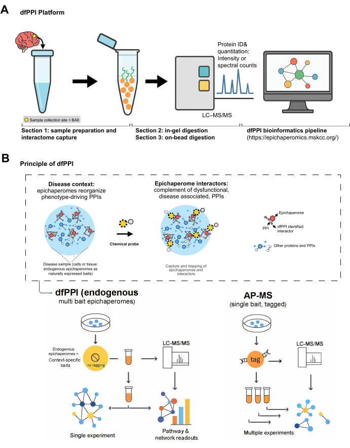
Figure 1: Overview of the dfPPI platform. (A) The dfPPI (dysfunctional Protein-Protein Interactome) platform enables the identification of disease-specific PPI network dysfunctions through a chemoproteomic workflow. Section 1 involves sample preparation and interactome capture using epichaperome-targeting chemical probes immobilized on affinity matrices (e.g., PU-beads). Sections 2 and 3 outline two compatible digestion workflows-on-bead or in-gel-followed by label-free LC-MS/MS for interactome identification. Computational analyses, including statistical modeling and pathway enrichment, are performed using the dfPPI bioinformatics pipeline, which is not covered in this protocol but is freely available at https://epichaperomics.mskcc.org/. (B) Principle of dfPPI. In disease-relevant contexts, endogenous epichaperomes form supramolecular scaffolds that reorganize PPI networks. Epichaperome-directed chemical probes (e.g., PU-beads or equivalent) capture these scaffolds together with their bound interactors directly from intact cells or from native lysates, yielding a multi-bait pull-down in a single experiment. Matched controls (e.g., inert-bead control and/or competition with free probe) can be processed in parallel. Captured material is eluted and digested on-bead or in-gel, analyzed by LC-MS/MS, and proteins are quantified (intensity or MS/MS spectral counts). The resulting interactome is used to compute differential interactors across conditions and to perform pathway/network enrichment, revealing context-specific PPI dysfunction at the systems level. The workflow requires no genetic tagging or overexpression, is compatible with both cells and tissues, and scales to cohort studies. Conversely, traditional affinity-purification-MS centers on one tagged bait at a time, producing a local neighborhood per construct and typically requiring many constructs/runs to sample a network. In contrast, dfPPI uses endogenous epichaperomes as the bait, capturing many dysfunctional PPIs simultaneously from the native system, which accelerates the discovery of disease-specific network rewiring and provides pathway-level readouts from a single capture. Please click here to view a larger version of this figure.

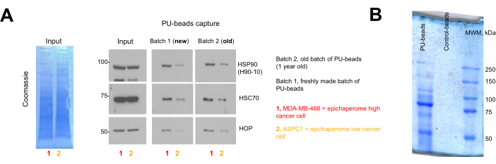
Figure 2: PU-bead lot validation and capture specificity. (A) Biological specificity and lot-to-lot consistency. MDA-MB-468 (epichaperome-high) and ASPC1 (epichaperome-low) cells were lysed in native buffer (20 mM Tris, pH 7.4; 20 mM KCl; 5 mM MgCl₂; 0.01% NP-40; protease/phosphatase inhibitors). For each capture, 40 µL of PU-bead slurry was incubated with 250 µg of total protein (1 µg/µL) for 3 h at 4 °C with rotation. Beads were washed in native buffer; complexes were denatured/eluted in ~100 µL of SDS sample buffer. 5-10 µL of each eluate was resolved by SDS-PAGE and immunoblotted for HSP90, HSC70, and HOP. Input lysates are shown for reference. Two PU-bead lots (Batch 1, fresh; Batch 2, aged) yield strong enrichment in MDA-MB-468 and minimal signal in ASPC1, demonstrating preserved specificity and lot consistency. (B) Global cargo versus control beads. MDA-MB-468 lysates were processed as in (A) with either PU-beads or matched control beads. ~20 µL of each eluate was loaded, separated by SDS-PAGE, and Coomassie-stained. PU-beads recover a complex, high-MW cargo characteristic of epichaperome-bound assemblies, whereas control beads show minimal background. Molecular-weight markers (kDa) are indicated. Please click here to view a larger version of this figure.

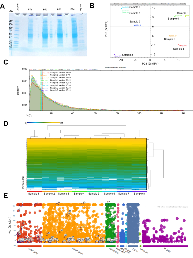
Figure 3: Representative results from dfPPI affinity capture, interactome identification, and bioinformatics analyses. (A) Coomassie-stained SDS-PAGE gel of proteins eluted from PU-bead affinity captures of epichaperome-bound interactomes from four representative human brain samples (PT1-PT4). Bead-bound protein assemblies were denatured by boiling in SDS sample buffer, resolved by SDS-PAGE, and stained to assess interactome recovery across molecular weights. Each sample was loaded into a separate lane, with an empty lane between samples to minimize cross-contamination; a faint signal occasionally observed in these empty lanes reflects minor sample spillover during electrophoresis. These gels are representative of samples submitted to the MS facility, where each lane was sectioned into five slices for in-gel digestion and protein identification by MS. (B) Principal component analysis (PCA) of identified protein intensities from on-bead digested epichaperome interactomes from eight representative murine brain samples (run in duplicate) reveals tight clustering of technical replicates and clear biological separation along PC1 and PC2. This confirms high technical reproducibility and sufficient biological variance for robust dfPPI analysis. The data structure demonstrates that interaction-level differences-not technical artifacts-drive sample separation, providing a strong foundation for downstream differential interactome modeling without requiring artificial normalization. (C) Coefficient of variation (CV) distributions for precursor ion intensities across the eight sample groups show consistently low variance, with median CVs ranging from 9.7% to 11.9% (indicated by vertical dashed lines). These low CVs highlight the reproducibility and robustness of the MS detection and quantification pipeline. The consistency supports the use of raw intensity or MS/MS values as reliable inputs for dfPPI analysis, where variance in interaction strength-not global protein expression-is the biological signal of interest. (D) Hierarchical clustering heatmap of log₂-transformed protein intensity values across all samples (with technical duplicates shown). Samples cluster by biological origin rather than replicate, confirming robust capture of epichaperome-bound interactomes and preservation of biologically relevant variance. Broad dynamic range and consistent detection across proteins further support dataset quality for dfPPI analysis. Scale bar represents log₂-transformed protein intensity values, ranging from 2 (blue, low abundance) to 14 (yellow, high abundance). (E) Manhattan plot of pathway enrichment analysis performed on differentially interacting proteins identified by dfPPI. Enrichment was conducted using g:Profiler, and significant terms are plotted by −log₁₀(p-value), colored by annotation source: GO Molecular Function (GO:MF), GO Biological Process (GO:BP), GO Cellular Component (GO:CC), KEGG, Reactome, WikiPathways, and Human Phenotype Ontology (HP). This output represents the core utility of dfPPI: uncovering biologically meaningful functional pathways perturbed through epichaperome-driven interactome remodeling. The broad annotation coverage underscores the systems-level insight achievable through this approach. Please click here to view a larger version of this figure.

Method	What it captures	Major strengths	Key limitations	Typical use	Scalability (cohorts)
AP-MS (affinity purification–MS)	Direct/near-direct interactors of a single bait	High specificity; quantitative; good for complex composition	Requires bait/tag/antibody; one bait at a time; may miss transient/weak	Define partners of a protein of interest	Low–moderate (many baits needed)
Proximity labeling (e.g., BioID/APEX variants)	Proteins in the nano-scale vicinity of a bait over time	Captures transient/weak neighbors; works in living cells	Genetic engineering; off-target labeling; parameter-heavy	Local neighborhood maps; dynamics	Low–moderate (engineering per bait)
XL-MS (cross-linking MS)	Spatial proximities/contacts within/between proteins	Structural restraints; captures transient contacts	Complex analysis; lower proteome breadth; sample-specific	Structural/contextual topology	Low (specialized)
Co-fractionation/MS (CF-MS)	Co-elution of native assemblies	No tagging; native assemblies	Labor-intensive; complex inference; limited sensitivity	Global complex landscape	Moderate
CETSA/TPP	Co-stability/co-aggregation profiles	Label-free; native conditions	Indirect for PPIs; solubility constraints	Target engagement; thermal shifts	Moderate
dfPPI (epichaperomics)	Network-level interaction rewiring captured by endogenous epichaperomes as multiplex baits	Endogenous; no tagging; one capture interrogates thousands of dysfunctional PPIs; pathway/network readouts; tissue-compatible; cohort-friendly	Applicable only to disease context; specialized probes (PU-beads, YK5-B); not intended for generic complex discovery	Disease-context interactome remodeling, pathway prioritization, hypothesis generation	High (hundreds of samples feasible)

Table 1: Comparison of PPI-mapping approaches and dfPPI. Please click here to download this Table.

Supplementary File 1: Full Spectronaut parameter settings. Please click here to download this File.

Discussion

The protocol described here enables mapping of dysfunctional PPIs in native biological samples using the dfPPI platform. Unlike traditional methods that infer dysfunction from abundance or expression changes, this platform captures network rewiring at the structural level by isolating disease-specific interactors through affinity purification with epichaperome-targeting probes, followed by label-free intensity-based quantitative MS. Although the current application focuses on post-mortem brain tissue, the method is broadly applicable to other sample types and disease models, including cultured cells and tissues from models of cancer, neurodegeneration, and immune dysfunction^{16,17,18,19,20,22,23}.

dfPPI relies on probes that kinetically select epichaperomes and trap the assemblies with their bound interactors. PU-beads (derived from epichaperome-binding chemotypes such as PU-H71/PU-AD) engage HSP90-nucleated epichaperomes non-covalently but with long residence time, a hallmark of kinetic selectivity for the epichaperome conformation over conventional chaperone complexes²³. YK5-B is a biotinylated, covalent probe directed to HSC70 within epichaperomes, enabling in-cell capture prior to lysis and preserving endogenous PPIs¹⁷. Selectivity stems from disease-associated PTMs that remodel HSP90/HSC70 conformations and pocket chemistry and stabilize epichaperome assemblies^14,23,43,44; these changes yield high-affinity, slow k_off binding for PU-type noncovalent probes⁴⁵ (and enable covalent capture with HSC70-directed YK5-B), thereby kinetically retaining epichaperome complexes and co-isolating their direct and indirect interactors for LC-MS/MS. In practice, PU-beads are optimal for lysate/homogenate workflows, whereas YK5-B supports live-cell capture; both retain context-dependent assemblies that can be identified by LC-MS/MS and used for downstream dfPPI analysis.

For dfPPI, specialized expertise in chemistry is required to synthesize the capture probes. However, this requirement is not unique to dfPPI: widely used PPI methods (AP-MS, proximity labelling, XL-MS) also rely on specialized skills-e.g., cloning/engineering tagged baits, stable cell line generation, labelling/crosslinking optimization, and complex bioinformatic pipelines. In contrast, dfPPI avoids genetic manipulation and bait overexpression, operates directly on native cells or tissues (including scarce clinical biospecimens), and uses standard affinity-capture and LC-MS workflows already routine in proteomics cores. To lower adoption barriers, validated PU-beads and matched control beads are available via MTA from the Chiosis laboratory, and handling/QA steps are fully specified in steps 1.3 and 1.4. Finally, analysis is supported by a web-based dfPPI app that implements the required statistics and pathway/network readouts, reducing bioinformatics burden (i.e., for users with no coding background and only basic bioinformatics skills).

AP-MS, XL-MS, proximity labelling, co-fractionation, and CETSA/TPP each answer different questions (direct binders, spatial proximity, neighborhood labelling, co-assembly, or thermal co-stability). dfPPI is the method of choice when the goal is to map endogenous, context-dependent rewiring in disease-especially in native tissues or large clinical cohorts where genetic tagging isn't feasible, and when pathway/network-level readouts from a single capture are desired. dfPPI uses epichaperomes as multiplex baits to capture coordinated interaction changes across many proteins in one pull-down, enabling scalable LC-MS/MS identification and pathway-centric analysis from primary material. In practice, dfPPI can seed downstream, bait-focused validation (e.g., AP-MS on specific nodes), while traditional methods can refine topology (direct contacts, spatial constraints) for complexes highlighted by dfPPI. See Table 1 for a side-by-side comparison.

Several critical steps influence the success of the workflow. First, high-quality protein extracts are essential. This requires careful handling of tissues or cells-ideally snap-frozen and stored at -80 °C-to minimize proteolysis and preserve native complexes. The inclusion of both protease and phosphatase inhibitors is non-negotiable: epichaperome integrity, which acts as the functional "bait" in this assay, depends on specific post-translational modifications of core components such as HSP90^23,43. For instance, phosphorylation of Ser226 and Ser255 is essential for stabilizing the epichaperome conformation and preserving its scaffolding function²³. Omission of phosphatase inhibitors risks structural collapse and loss of biological specificity.

Another key determinant is the quality and handling of the PU-beads affinity matrix. Beads should be stored in 100% isopropanol at -20 °C and used within a defined activity window, ideally within 1-2 years. Activity should be validated prior to critical experiments, as aged beads may exhibit reduced binding capacity or increased nonspecific interactions. Incubation time and protein input must also be optimized: over-incubation may elevate background, whereas insufficient protein input may compromise depth of detection. We recommend 3 h incubations and pilot pull-downs to calibrate the appropriate input for each sample type.

Two digestion strategies are compatible with this protocol: on-bead and in-gel. While both workflows yield reproducible results, each offers trade-offs. In-gel digestion may introduce contaminants such as keratin and requires additional handling steps. On-bead digestion streamlines the workflow and is generally preferred when sample throughput or input amount is limiting. However, protease amounts must be calibrated based on total protein input: although the method is designed for 750 ng of trypsin, incomplete digestion may occur if protein levels are high, leading to missed cleavages and reduced peptide recovery. It is advisable to assess digestion efficiency and adjust enzyme input accordingly. All digestion steps should be performed in low-binding tubes using freshly prepared, contamination-free reagents to ensure consistency and minimize background.

Protein loading per LC-MS injection depends on the capture workflow, peptide yield, and column capacity. For on-bead digests analyzed on standard nano-LC C18 columns (~50-75 µm ID, ~15-25 cm), we typically load 300-500 ng per injection; we have not observed performance gains above ~400-500 ng, while higher loads risk ion suppression and peak broadening. For in-gel workflows (e.g., five slices per lane), we generally inject ~25% of the desalted material per slice per replicate and retain ~50% as backup for reinjection if needed. In all cases, measure peptide concentration prior to injection, verify linear response with a QC digest, and tune the load so chromatographic peak shape and identification depth are maintained without overloading.

Label-free quantification via DIA is widely used in proteomics due to its reproducibility and depth⁴⁶. However, in the context of affinity capture experiments such as this-where the goal is to identify proteins interacting with epichaperome scaffolds rather than measure global protein abundance-normalization strategies like MaxLFQ are not appropriate. These approaches assume uniform input and proteome-wide similarity, which are violated by the enrichment step intrinsic to this protocol. Instead, intensity values or MS/MS spectral counts provide sufficient and biologically meaningful quantification for downstream functional analysis. These metrics reflect the relative interaction strength or frequency of proteins with epichaperomes across conditions. As demonstrated in prior studies^16,17,18,20, these values are well-suited for systems-level interactome analyses such as dfPPI, which identify altered biological pathways without relying on proteome-wide normalization. By preserving the true biological variance introduced by disease or treatment, intensity- or MS/MS-based quantification enables accurate and robust mapping of PPI network dysfunctions.

Although affinity capture reduces the search space versus whole lysate, dfPPI pull-downs still contain hundreds to thousands of proteins spanning a wide dynamic range, plus co-enriched background. For cohort-scale comparisons, DDA's stochastic precursor selection leads to run-to-run missing values and variable sampling of low-abundance interactors¹⁸. DIA systematically fragments all ions in predefined windows, providing greater depth, fewer missing values, and higher run-to-run reproducibility-properties that are crucial when downstream inference is pathway/network-level rather than single-protein. This is why we standardize on DIA for dfPPI.

As with all affinity capture methods, nonspecific protein binding is an inherent consideration. Proteins may be retained due to stickiness to the resin, high abundance, or aggregation. While such nonspecific interactors can appear in the pull-down eluate, their presence does not undermine the downstream analytical objective of this protocol¹⁷. The dfPPI workflow is not designed to define binary interactions but rather to extract patterns of PPI rewiring at the systems level. Functional enrichment analyses are performed on differential interactors and leverage network-based statistics to reveal coordinated pathway-level alterations. As demonstrated in previous work¹⁷, this systems-level approach minimizes the impact of isolated nonspecific proteins and allows robust biological conclusions to emerge from cohort-level data.

Compared to conventional interactome mapping approaches-such as co-immunoprecipitation, proximity labelling, or cross-linking-the dfPPI platform offers a distinct advantage: it captures functional interactome remodeling under disease-relevant conditions without requiring bait engineering or overexpression. Because the method isolates protein complexes formed around supramolecular epichaperomes, it detects emergent protein assemblies that are not present in healthy systems, enabling the discovery of novel disease drivers. The approach is scalable and adaptable across tissues, species, and disease states, and it has already provided unique insights into proteome remodeling in cancer and neurodegeneration. As such, this method offers a powerful tool for uncovering functional networks disrupted in human disease.

Beyond the exemplars here, dfPPI is well positioned for (i) large clinical cohorts to stratify patients by network dysfunction and to discover pharmacodynamic biomarkers that report on target engagement and pathway correction; (ii) longitudinal sampling (e.g., pre/post therapy, disease staging) to track rewiring trajectories and predict responders; (iii) integration with phosphoproteomics and other PTM-aware omics to link interaction-state changes to upstream signaling; (iv) spatially resolved captures from microdissected regions (tumor-normal interfaces, brain subregions) to map local network pathobiology; (v) perturbation screens (genetic or compound) where dfPPI readouts nominate actionable nodes and mechanisms-of-action; and (vi) graph/AI modeling that learns disease-specific network features from dfPPI maps for prognosis and therapeutic design. Methodologically, miniaturization, automation (e.g., 96-well formats), and standardized QC will enable high-throughput pipelines for translational studies and clinical trials. Finally, dfPPI outputs can seed targeted follow-ups-AP-MS, XL-MS, or proximity labelling-to resolve topology of prioritized modules, underscoring the method's complementarity within the interactomics toolkit.

Materials

List of materials used in this article

Name	Company	Catalog Number	Comments
2-mercaptoethanol	Sigma-Aldrich	M6250	Toxic, Combustible
Acetonitrile (ACN) Optima	Fisher Scientific	A955-1	LC/MS grade (Flammable)
Affi-Gel 10 activated affinity chromatography media	Bio-Rad	1536099	Used to make PU-beads and control beads (Flammable)
Ammonium Bicarbonate (ABC)	Sigma-Aldrich	09830-500G
Aurora Ultimate 25x75 C18 UHPLC column	IonOpticks	AUR3-25075C18-CSI
Autoradiographic film	EWEN-PARKER X-RAY CORP	EBA45	Alternative for chemiluminescent signal detection after Western blot
Biomasher micro tissue homogenizer	DWK Life Sciences Kimble	7496250010	Used for homogenizing frozen brain tissue for protein extraction
Bromophenol blue	Fisher Bioreagent	BP115-25
Centrifuge for 1.5 mL tubes	Eppendorf	5424
Centrifuge for 1.5 mL tubes	Eppendorf	5417R	With temperature control
Centrifuge for 15-50 mL tubes	Eppendorf	5810R	Used for conical tubes
ChemiDoc MP imaging system	Bio-Rad	17001402	Used for gel/blot densitometry
Column oven	Sonation GmBH, Germany	ES071/ES072	Maintains nanoLC column at 50 °C for consistent retention
Conical tubes (15 mL)	Fisher Scientific	352096
Control-beads	Chiosis Lab	N/A	Taldone et al. (PMID: 21459002)
Coomassie G-250 stain (Bio-safe)	Bio-Rad	1610786
Dark Eppendorf tubes (1.5 mL)	USA Scientific	1415-2507
Dithiothreitol (DTT)	Roche	10197777001	Irritant
Easy nLC 1000	Thermo Fisher Scientific	Easy nLC 1000	LC system used with Q Exactive HF
Empore Solid Phase Extraction Disks	3M Company	2215-C18 (Octadecyl)	Used to prepare StageTips for peptide desalting; Activated with 100% Methanol
Enhanced chemiluminescence (ECL) kit	Thermo Fisher Scientific	32209
Eppendorf tubes (1.5 mL)	Fisher Scientific	05-408-129
Formic Acid (FA) Optima	Fisher Scientific	A117-10X1AMP	LC/MS-grade
g:Profiler (e111_eg58_p18_f463989d)	BIIT Group-Tartu Ülikool	https://biit.cs.ut.ee/gprofiler/gost	Pathway enrichment
Glycerol	Fisher Bioreagent	BP229-1	Molecular biology grade
Glycine	Fisher Bioreagent	BP381-5	Crystalline Powder
Goat anti-mouse HRP-conjugated secondary antibody (RRID: AB_2619742)	Sothern Biotech	1030-05	Secondary for the H90-10 antibody
Goat anti-rabbit HRP-conjugated secondary antibody (RRID: AB_2632593)	Sothern Biotech	4010-05	Secondary for the HSP90α and HOP antibodies
Goat anti-rat HRP-conjugated secondary antibody (RRID: AB_2716837)	Sothern Biotech	3030-05	Secondary for the HSC70 antibody
Heated orbital shaker	Eppendorf	ThermoMixer C (2231001127)
HeLa protein digest standard-Pierce	Thermo Fisher Scientific	88329	Used for LC-MS QC assessment
HOP antibody (RRID: AB_10828378)	Cell Signaling	5670	For PU-beads QC
HSC70 antibody (RRID: AB_10617277)	Enzo	SPA-815	For PU-beads QC
HSP90 (H90-10) antibody (RRID: AB_854214)	StressMarq	SMC-107	For PU-beads QC
HSP90 alpha antibody (RRID: AB_303423)	Abcam	Ab2928	For normalization as per Section 1.2
Human cell line: ASPC1 (RRID:CVCL_0152)	ATCC	CRL-1682	Control cell line, epichaperome low/chaperone high
Human cell line: MDA-MB-468 (RRID: CVCL_0419)	ATCC	HTB-132	Control cell line, epichaperome high/chaperone high
ImageJ (v1.54p)	Wayne Rasband	https://imagej.net/ij/	Densitometry
Iodoacetamide (IAA)	Sigma-Aldrich	I1149-5G	Toxic
Low-protein binding microcentrifuge tubes	Sarstedt	72.706.600
Lys-C protease	Promega	VA1170	LC/MS-grade
Magnesium Chloride	Sigma-Aldrich	63068	Molecular biology grade
MaxQuant (v2.1.1.0)	Max-Planck-Institute of Biochemistry	https://www.maxquant.org/	MaxDIA workflow for peptide/protein identification and label-free intensity-based quantification
Methanol	Fisher Chemical	A454-4	HPLC grade, flammable, toxic
Mini Protease Inhibitor Cocktail tablet (Complete)	Roche	4693124001
Mini Trans Blot Electrophoretic Transfer Cell	Bio-Rad	1703930
Mini-gel electrophoresis tank	Thermo Fisher Scientific	A25977	Used for Novex precast gels
Mini-PROTEAN Tetra Vertical Electrophoresis Cell	Bio-Rad	1658004	Used for Mini-PROTEAN Precast Protein Gels or hand cast gels
Mini-PROTEAN TGX Precast Protein Gels (4–20%)	Bio-Rad	4561094
NanoDrop	Agilent	BioTek Synergy H1	Used to estimate peptide concentration before LC-MS injection
NanoElute 2	Bruker	https://flextra.hu/images/keszulekek/daltonics/nanoelute-brosura_eng.pdf	Used in diaPASEF workflow
Nanospray Flex source	Thermo Fisher Scientific	ES071	For nanospray ESI coupling
New Objective PicoTip Emmiter/PicoFrit SELF/P	New Objective Inc.	PF360-75-10-N-5	Packed with C18 slurry to 20 cm in length
Nitrocellulose membrane	Cytiva Amersham	10600006
Nonfat dry milk	Lab Scientific	M0841
Novex 8% Tris-Glycine precast gels	Thermo Fisher Scientific	XP00080BOX
NP-40	Roche	11754599001
Phosphate buffered saline (PBS)	Gibco	10010023
PhosSTOP phosphatase inhibitor cocktail tablet	Roche	4906837001
Pierce BCA protein assay kit	Thermo Fisher Scientific	23225
Plastic containers	Fisher Scientific	FB0875711A
Platform rocker	Corning	6705
Potassium chloride	Fisher Bioreagent	BP366-1	White Crystals
PowerPac Universal Power Supply	Bio-Rad	1645070
Precision Plus Protein Kaleidoscope Prestained Protein Standard	Bio-Rad	1610375
PU-beads	Chiosis Lab	N/A	Taldone et al. (PMID: 21459002)
Q Exactive HF Orbitrap mass spectrometer	Thermo Fisher Scientific	https://assets.thermofisher.com/TFS-Assets/CMD/brochures/BR-64052-LC-MS-Q-Exactive-HF-Orbitrap-BR64052-EN.pdf	Used for DIA-MS
ReproSil-Pur 120 C18-AQ, 3 µm	Dr. Maisch GmbH, Germany	R13.aq	Silica media for peptide separation; Slurry of powder/Methanol (1:3, v/v)
Rotation unit (end-over-end rotator)	Barnstead International	400110
Sep-Pak C18 Cartridges (100 mg)	Waters Corporation	WAT023590
Sodium dodecyl sulfate (SDS)	Fisher Bioreagent	BP166-500	Electrophoresis grade
Sonicator	Branson	2510
SpectraMax Paradigm Multi-Mode Microplate reader	Molecular Devices	SpectraMax Paradigm
Spectronaut	Biognosys	https://biognosys.com/software/spectronaut/	directDIA workflow
SpeedVac concentrator	Thermo Fisher Scientific	Savant SPD111V
Suction vacuum	Cardinal Health	CDL-65651-320
TimsTOF HT mass spectrometer	Bruker	https://www.bruker.com/en/products-and-solutions/mass-spectrometry/timstof/timstof-ht.html	Used for diaPASEF analysis
Trifluoracetic Acid (TFA) Optima	Sigma-Aldrich	T6508-10AMP	LC/MS-grade (Corrosive, combustible)
Tris	Fisher Bioreagent	BP152-5	Crystalline powder; Molecular biology grade
Tris, pH 6.8 (1 M)	Teknova	T1068
Tris, pH 7.5 (1 M)	Fisher Bioreagent	BP1757-500	Molecular biology grade
Tris-buffered saline (20x TBS) buffer	VWR, Life science	97064-338
Tris-Glycine-SDS (TGS 10x) running gel buffer	Fisher Bioreagent	BP13414	Electrophoresis
Trypsin	Promega	V5111	Sequencing grade
Trypsin Gold	Promega	V5280
Tween 20	Fisher Bioreagent	BP337-100
Urea	Sigma-Aldrich	U0631-500G
Vortex	Fisher Scientific	02-215-414
Water	Fisher Scientific	W6-1	LC/MS grade

References

- Liu, Z., Miller, D., Li, F., Liu, X., Levy, S. F. A large accessory protein interactome is rewired across environments. Elife. 9, e62365(2020).
- Omranian, S., Nikoloski, Z., Grimm, D. G. Computational identification of protein complexes from network interactions: Present state, challenges, and the way forward. Comput Struct Biotechnol J. 20, 2699-2712 (2022).
- Ginsberg, S. D., Sharma, S., Norton, L., Chiosis, G. Targeting stressor-induced dysfunctions in protein-protein interaction networks via epichaperomes. Trends Pharmacol Sci. 44 (1), 20-33 (2023).
- Nussinov, R. Pioneer in molecular biology: Conformational ensembles in molecular recognition, allostery, and cell function. J Mol Biol. 437 (11), 169044(2025).
- Lacoste, J., et al. Pervasive mislocalization of pathogenic coding variants underlying human disorders. Cell. 187 (23), 6725-6741.e13 (2024).
- Liu, X., Abad, L., Chatterjee, L., Cristea, I. M., Varjosalo, M. Mapping protein-protein interactions by mass spectrometry. Mass Spectrom Rev. , (2024).
- Luck, K., Sheynkman, G. M., Zhang, I., Vidal, M. Proteome-scale human interactomics. Trends Biochem Sci. 42 (5), 342-354 (2017).
- Greenblatt, J. F., Alberts, B. M., Krogan, N. J. Discovery and significance of protein-protein interactions in health and disease. Cell. 187 (23), 6501-6517 (2024).
- Gonzalez-Avendano, M., Lopez, J., Vergara-Jaque, A., Cerda, O. The power of computational proteomics platforms to decipher protein-protein interactions. Curr Opin Struct Biol. 88, 102882(2024).
- Komives, E. A., Chiosis, G. Editorial overview: Protein networks in health and disease. Curr Opin Struct Biol. 90, 102953(2025).
- Botticelli, L., et al. Chemical cross-linking and mass spectrometry enabled systems-level structural biology. Curr Opin Struct Biol. 87, 102872(2024).
- Chakrabarty, S., Wang, S., Roychowdhury, T., Ginsberg, S. D., Chiosis, G. Introducing dysfunctional protein-protein interactome (dfppi) - a platform for systems-level protein-protein interaction (ppi) dysfunction investigation in disease. Curr Opin Struct Biol. 88, 102886(2024).
- Pasala, C., et al. Epichaperomes: Redefining chaperone biology and therapeutic strategies in complex diseases. RSC Chem Biol. 6 (5), 678-698 (2025).
- Chu, F., Sharma, S., Ginsberg, S. D., Chiosis, G. PTMs as molecular encoders: Reprogramming chaperones into epichaperomes for network control in disease. Trends Biochem Sci. , (2025).
- Chiosis, G., Digwal, C. S., Trepel, J. B., Neckers, L. Structural and functional complexity of hsp90 in cellular homeostasis and disease. Nat Rev Mol Cell Biol. 24 (11), 797-815 (2023).
- Rodina, A., et al. The epichaperome is an integrated chaperome network that facilitates tumour survival. Nature. 538 (7625), 397(2016).
- Rodina, A., et al. Systems-level analyses of protein-protein interaction network dysfunctions via epichaperomics identify cancer-specific mechanisms of stress adaptation. Nat Commun. 14 (1), 26(2023).
- Inda, M. C., et al. The epichaperome is a mediator of toxic hippocampal stress and leads to protein connectivity-based dysfunction. Nat Commun. 11 (1), 19(2020).
- Joshi, S., et al. Pharmacologically controlling protein-protein interactions through epichaperomes for therapeutic vulnerability in cancer. Commun Biol. 4 (1), 20(2021).
- Bay, S., et al. Systems-level interactome mapping reveals actionable protein network dysregulation across the alzheimer's disease spectrum. Res Sq. , (2025).
- Moulick, K., et al. Affinity-based proteomics reveal cancer-specific networks coordinated by HSP90. Nat Chem Biol. 7 (11), 818-826 (2011).
- Kishinevsky, S., et al. Hsp90-incorporating chaperome networks as biosensor for disease-related pathways in patient-specific midbrain dopamine neurons. Nat Commun. 9, 15(2018).
- Roychowdhury, T., et al. Phosphorylation-driven epichaperome assembly is a regulator of cellular adaptability and proliferation. Nat Commun. 15 (1), 8912(2024).
- Roychowdhury, T., et al. Use of native-page for the identification of epichaperomes in cell lines. Methods Mol Biol. 2693, 175-191 (2023).
- Taldone, T., et al. synthesis, and evaluation of small molecule HSP90 probes. Bioorg Med Chem. 19 (8), 2603-2614 (2011).
- Meier, F., Park, M. A., Mann, M. Trapped ion mobility spectrometry and parallel accumulation-serial fragmentation in proteomics. Mol Cell Proteomics. 20, 100138(2021).
- Rappsilber, J., Mann, M., Ishihama, Y. Protocol for micro-purification, enrichment, pre-fractionation and storage of peptides for proteomics using stagetips. Nat Protoc. 2 (8), 1896-1906 (2007).
- Kovalchuk, S. I., Jensen, O. N., Rogowska-Wrzesinska, A. Flashpack: Fast and simple preparation of ultrahigh-performance capillary columns for LC-MS. Mol Cell Proteomics. 18 (2), 383-390 (2019).
- Sinitcyn, P., et al. Maxdia enables library-based and library-free data-independent acquisition proteomics. Nat Biotechnol. 39 (12), 1563-1573 (2021).
- DiscoveryLibraries. , The Max Planck Institute of Biochemistry. Available from: https://datashare.biochem.mpg.de/s/qe1IqcKbz2j2Ruf?dir=/DiscoveryLibraries (2025).
- Rappsilber, J., Ishihama, Y., Mann, M. Stop and go extraction tips for matrix-assisted laser desorption/ionization, nanoelectrospray, and LC/MS sample pretreatment in proteomics. Anal Chem. 75 (3), 663-670 (2003).
- Meier, F., et al. Diapasef: Parallel accumulation-serial fragmentation combined with data-independent acquisition. Nat Methods. 17 (12), 1229-1236 (2020).
- Lou, R., et al. Benchmarking commonly used software suites and analysis workflows for dia proteomics and phosphoproteomics. Nat Commun. 14 (1), 94(2023).
- Demichev, V., et al. Dia-pasef data analysis using fragpipe and dia-nn for deep proteomics of low sample amounts. Nat Commun. 13 (1), 3944(2022).
- Wen, C., et al. Evaluation of DDA library-free strategies for phosphoproteomics and ubiquitinomics data-independent acquisition data. J Proteome Res. 22 (7), 2232-2245 (2023).
- Bowler-Barnett, E. H., et al. Uniprot and mass spectrometry-based proteomics-A 2-way working relationship. Mol Cell Proteomics. 22 (8), 100591(2023).
- Demichev, V., Messner, C. B., Vernardis, S. I., Lilley, K. S., Ralser, M. Dia-nn: Neural networks and interference correction enable deep proteome coverage in high throughput. Nat Methods. 17 (1), 41-44 (2020).
- Wang, T., Digwal, C. S., Alam, A., Chiosis, G. R. script epichaperomics - systems-level analyses of protein-protein interaction network dysfunctions via epichaperomics identify cancer-specific mechanisms of stress adaptation. Zenodo. , https://doi.org/10.5281/zenodo.7416220 (2022).
- Chaperomics_ad_2019. , Chiosislab. https://github.com/chiosislab/Chaperomics_AD_2019 (2019).
- Chaperomics_controllability_2020. , Chiosislab. https://github.com/chiosislab/Chaperomics_controllability_2020 (2019).
- Alam, A., Wang, T., Chiosis, G. Cytoscape files - systems-level analyses of protein-protein interaction network dysfunctions via epichaperomics identify cancer-specific mechanisms of stress adaptation [data set]. Zenodo. , https://doi.org/10.5281/zenodo.7433980 (2022).
- Kolberg, L., et al. G:Profiler-interoperable web service for functional enrichment analysis and gene identifier mapping (2023 update). Nucleic Acids Res. 51 (W1), W207-W212 (2023).
- Yan, P. R., et al. Molecular stressors engender protein connectivity dysfunction through aberrant n-glycosylation of a chaperone. Cell Reports. 31 (13), 27(2020).
- Castelli, M., et al. How aberrant n-glycosylation can alter protein functionality and ligand binding: An atomistic view. Structure. 31 (8), 987-1004.e8 (2023).
- Sharma, S., et al. Unraveling the mechanism of epichaperome modulation by zelavespib: Biochemical insights on target occupancy and extended residence time at the site of action. Biomedicines. 11 (10), 2599(2023).
- Guzman, U. H., et al. Ultra-fast label-free quantification and comprehensive proteome coverage with narrow-window data-independent acquisition. Nat Biotechnol. 42 (12), 1855-1866 (2024).
Reprints and Permissions