Back to chapter

12.6:

Chi-square Analysis

JoVE Core
Molecular Biology
A subscription to JoVE is required to view this content.  Sign in or start your free trial.
JoVE Core Molecular Biology
Chi-square Analysis

Languages

Share

Mendel hypothesized that the phenotypic ratio of a monohybrid cross between individuals with a dominant trait, like purple flowers, and a recessive trait, like white flowers, would be approximately three to one provided the alleles are independently assorted.

When there is an assumption that data will fit a certain ratio, like Mendel’s 3:1 prediction, a null hypothesis is established. The null hypothesis assumes that there is no real difference between the expected and observed values and that any apparent differences are due to chance.

Consider a monohybrid cross between twenty tall plants and twenty short plants. The F2 generation of this cross yields 33 tall plants and 7 short plants. This is the observed value.

To test the null hypothesis, a chi-square analysis can be performed. First, create a table with three columns: phenotype, observed value, and expected value. The phenotype and observed values are already known, but the expected values must be calculated.

Calculate the expected values by dividing the total number of plants observed with the total number of expected plants – that is three plus one equals four. So, forty divided by four is ten.

Ten represents the “one” of the expected three to one frequency. Hence, there are ten plants with the recessive “short” gene.

Now, multiply ten by three to obtain the “three” of the expected three to one frequency. Thus, there are thirty plants with the dominant “tall” gene.

Calculate the difference between the observed and expected value in each row and square the results.

Then, divide this value by the expected value in each row and add them all together to obtain the chi-squared value – 1.2.

The degree of freedom, which is defined as the number of values that can vary in the final calculation of a statistic, must also be calculated. Obtain the degree of freedom using this formula, where n is the number of classes, or in this case phenotypes. Here, there is one degree of freedom.

Using the chi-squared value and degree of freedom, obtain the result on the probability chart. Here, 1.2 falls between 1.07 and 1.64. The p-values for these is 0.30 and 0.20, which is greater than 0.05. Thus, the null hypothesis is not rejected, indicating that the alleles for plant height are independently assorted.

12.6:

Chi-square Analysis

The chi-square test is a statistical hypothesis test. It is used to check whether there is a significant difference between an expected value and an observed value. In the context of genetics, it enables us to either accept or reject a hypothesis, based on how much the observed values deviate from the expected values.

The chi-square test was developed by Pearson in 1990.

The first step of performing a Chi-square analysis is to establish a null hypothesis, which assumes that there is no real difference between the expected value and the observed value. Any apparent deviations from the expected value are simply due to chance.

The null hypothesis is rejected if the probability value is less than 5%. Consider, for example, a cross in a plant species with yellow and green seeds. All the F1 generation plants had green seeds. Upon self-fertilization among the F1 generation, the expected value in F2 generation is 660 plants with green seeds and 220 plants with yellow seeds. However, the observed value in the F2 generation is 620 plants with green seeds and 260 plants with yellow seeds. Now chi-square is used to find out if the difference between observed and expected values are significant? Can we conclude that the observed inheritance follows Mendelian monohybrid cross?

 The chi-squared value is calculated using the formula given below:

Figure1

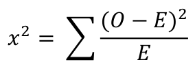
Where O is the observed value and E is the expected value.

The chi-square value is calculated as 9.69. To accept or reject the hypothesis, the degrees of freedom are required. The degree of freedom is the number of classes minus one. It refers to the values involved in the calculation that vary.

In the above example, two different colors of seeds are observed. So the degree of freedom will be 2 – 1 = 1. To check if the result is statistically significant, the calculated chi-square value and the degree of freedom are analyzed on the probability chart under α=0.05. The value from the table is 3.841. Since the chi-squared value 9.69 is greater than 3.841, we have statistically significant evidence to reject the null hypothesis. In other words, the differences observed between the experimental and expected values is due to chance alone.

Suggested Reading