Building an Enhanced Flight Mill for the Study of Tethered Insect Flight

Summary

This protocol uses three-dimensional (3D) printers and laser cutters found in makerspaces in order to create a more flexible flight mill design. By using this technology, researchers can reduce costs, enhance design flexibility, and generate reproducible work when constructing their flight mills for tethered insect flight studies.

Abstract

Makerspaces have a high potential of enabling researchers to develop new techniques and to work with novel species in ecological research. This protocol demonstrates how to take advantage of the technology found in makerspaces in order to build a more versatile flight mill for a relatively low cost. Given that this study extracted its prototype from flight mills built in the last decade, this protocol focuses more on outlining divergences made from the simple, modern flight mill. Previous studies have already shown how advantageous flight mills are to measuring flight parameters such as speed, distance, or periodicity. Such mills have allowed researchers to associate these parameters with morphological, physiological, or genetic factors. In addition to these advantages, this study discusses the benefits of using the technology in makerspaces, like 3D printers and laser cutters, in order to build a more flexible, sturdy, and collapsible flight mill design. Most notably, the 3D printed components of this design allow the user to test insects of various sizes by making the heights of the mill arm and infrared (IR) sensors adjustable. The 3D prints also enable the user to easily disassemble the machine for quick storage or transportation to the field. Moreover, this study makes greater use of magnets and magnetic paint to tether insects with minimal stress. Lastly, this protocol details a versatile analysis of flight data through computer scripts that efficiently separate and analyze differentiable flight trials within a single recording. Although more labor-intensive, applying the tools available in makerspaces and on online 3D modeling programs facilitates multidisciplinary and process-orientated practices and helps researchers avoid costly, premade products with narrowly adjustable dimensions. By taking advantage of the flexibility and reproducibility of technology in makerspaces, this protocol promotes creative flight mill design and inspires open science.

Introduction

Given how intractable the dispersal of insects is in the field, the flight mill has become a common laboratory tool to address an important ecological phenomenon - how insects move. As a consequence, since the pioneers of the flight mill^1,2,3,4 ushered in six decades of flight mill design and construction, there have been noticeable design shifts as technologies improved and became more integrated into scientific communities. Over time, automated data-collecting software replaced chart recorders, and flight mill arms transitioned from glass rods to carbon rods and steel tubing⁵. In the last decade alone, magnetic bearings replaced Teflon or glass bearings as optimally frictionless, and pairs between flight mill machinery and versatile technology have been proliferating as audio, visual, and layer fabrication technology become increasingly integrated into researchers' workflows. These pairings have included high-speed video cameras to measure wing aerodynamics⁶, digital-to-analog boards to mimic sensory cues for studying auditory flight responses⁷, and 3D printing to make a calibration rig to track wing deformation during flight⁸. With the recent rise of emerging technologies at makerspaces, particularly at institutions with digital media centers run by knowledgeable staff⁹, there are greater possibilities to enhance the flight mill to test a larger range of insects and to transport the device to the field. There is also a high potential for researchers to cross disciplinary boundaries and accelerate technical learning through production-based work^9,10,11,12. The flight mill presented here (adapted from Attisano and colleagues¹³) takes advantage of emerging technologies found in makerspaces to not only 1) create flight mill components whose scales and dimensions are fine-tuned to the project at hand but also 2) offer researchers an accessible protocol in laser cutting and 3D printing without demanding a high-budget or any specialized knowledge in computer-aided design (CAD).

The benefits of coupling new technologies and methods with the flight mill are substantial, but flight mills are also valuable stand-alone machines. Flight mills measure insect flight performance and are used to determine how flight speed, distance, or periodicity relates to environmental or ecological factors, such as temperature, relative humidity, season, host plant, body mass, morphological traits, age, and reproductive activity. Distinct from alternative methods like actographs, treadmills, and the video recording of flight movement in wind tunnels and indoor arenas¹⁴, the flight mill is notable for its ability to collect various flight performance statistics under laboratory conditions. This helps ecologists address important questions on flight dispersal, and it helps them progress in their discipline - whether that be integrated pest management^15,16,17, population dynamics, genetics, biogeography, life-history strategies¹⁸, or phenotypic plasticity^19,20,21,22. On the other hand, devices like high-speed cameras and actographs can require a strict, complicated, and expensive setup, but they can also lead to more fine-tuned movement parameters, such as wing-beat frequencies and insect photophase activity^23,24. Thus, the flight mill presented here serves as a flexible, affordable, and customizable option for researchers to investigate flight behavior.

Likewise, the incentive to integrate emerging technologies into ecologists' workflow continues to rise as questions and approaches to studying dispersal become more creative and complex. As locations that promote innovation, makerspaces draw in multiple levels of expertise and offer a low learning curve for users of any age to acquire new technical skills^10,12. The iterative and collaborative nature of prototyping scientific devices in the makerspace and through online open sources can accelerate the application of theory¹¹ and facilitate product development in the ecological sciences. Furthermore, increasing the reproducibility of scientific tools will encourage wider data collection and open science. This can help researchers standardize equipment or methods for measuring dispersal. Standardizing tools could further allow ecologists to unify dispersal data across populations in order to test metapopulation models that develop from dispersal kernels²⁵ or source-sink colonization dynamics²⁶. Much like how the medical community is adopting 3D printing for patient care and anatomy education²⁷, ecologists can use laser cutters and 3D printers to redesign ecological tools and education and, within the scope of this study, can design additional flight mill components, such as landing platforms or a flight mill arm that can move vertically. In turn, the customization, cost-effectiveness, and increased productivity offered by makerspace technology can help start up dispersal projects with a relatively low barrier for researchers who intend to develop their own tools and devices.

To construct this flight mill, there are also mechanical and instrumental limitations that can be considered by the maker. Magnets and 3D printed enhancements allow the flight mill to be essentially glueless, except for the construction of the cross brackets, and to be accommodable to insects of different sizes. However, as the mass and the strength of insects increase, insects may be more likely to dismount themselves while tethered. Strong magnets can be used at the cost of increased torsional drag, or ball bearings can replace magnetic bearings as a robust solution for flight testing insects that weigh several grams^28,29. Nevertheless, ball bearings can also present some problems, mainly that running prolonged experiments with high speeds and high temperatures can degrade the lubrication of ball bearings, which increases friction³⁰. Thus, users will have to discern which flight mill mechanics would best suit their insect(s) of study and experimental design.

Similarly, there are several ways to instrument a flight mill that is beyond this paper's considerations. The flight mill presented here uses IR sensors to detect revolutions, WinDAQ software to record revolutions, and programming scripts to process the raw data. Although it is easy-to-use, the WinDAQ software has a limited array of tools available. Users cannot attach comments to their corresponding channel, and they cannot be alerted if any component of the circuitry fails. These cases are solved by detecting and correcting them through code but only after data collection. Alternatively, users can adopt more than one software that offers customizable data collection features²⁸ or sensors that take direct speed and distance statistics, like bike milometers²⁹. However, these alternatives can bypass valuable raw data or diffuse functionality across too many software applications, which can make data processing inefficient. Ultimately, rather than refashioning flight mill instrumentation, this protocol offers robust programming solutions to present-day software limitations.

In this paper, a design for an enhanced simple flight mill is described to aid researchers in their dispersal studies and to encourage the incorporation of emerging technologies in the field of behavioral ecology. This flight mill fits within the constraints of an incubator, holds up to eight insects simultaneously, and automates data collection and processing. Notably, its 3D printed enhancements allow the user to adjust the mill arm and IR sensor heights to test insects of various sizes and to disassemble the device for quick storage or transportation. Thanks to institutional access to a communal makerspace, all enhancements were free, and no additional costs were accrued compared to the simple, modern flight mill. All software needed are free, the electronic circuitry is simple, and all scripts can be modified to follow the specific needs of the experimental design. Moreover, coded diagnostics allow the user to check the integrity and precision of their recordings. Lastly, this protocol minimizes the stress sustained by an insect by magnetically painting and tethering insects to the mill arm. With the assembly of the simple flight mill being already accessible, affordable, and flexible, the use of makerspace technologies to enhance the simple flight mill can grant researchers the space to overcome their own specific flight study needs and can inspire creative flight mill designs beyond this paper's considerations.

Protocol

1. Build the Flight Mill in a Makerspace

1. Laser cut and assemble the acrylic plastic support structure.
   1. Use 8 (304.8 mm x 609.6 mm x 3.175 mm) thick transparent acrylic sheets to construct the acrylic plastic support structure. Ensure that the material is not polycarbonate, which looks similar to acrylic but will melt instead of getting cut under the laser.
   2. Locate the laser cutter in the makerspace. This protocol assumes the makerspace has a laser cutter as referenced in the Table of Materials. For other laser cutters, read the laser cutter settings to determine what line color or thickness is needed to set the file lines to be laser cut or engraved (not to be rastered).
   3. Open Adobe Illustrator, Inkscape (free), or another vector graphics editor. Prepare a file that reads the acrylic support design in a vector format with the aforementioned lines shown in Figure 1. Create file lines in Adobe Illustrator in Red, Green, and Blue (RGB) mode with a line stroke of 0.0001 point where RGB Red (255, 0, 0) cuts lines and RGB Blue (0, 0, 255) etches lines.
   4. As a precaution, test and account for kerf for all slit and hole measurements. Design and test the kerf key (Supplemental Figure 1).
      ​NOTE: Kerf width can vary based on the beam width of the laser cutter, the width of the material, and the material type used.
   5. Save the acrylic support designs and kerf key as readable file types such as .ai, .dxf, or .svg files. To send the job to the laser cutter, print the file on the laser cutter's local machine and then open the laser software.
      NOTE: If printed correctly, all the vector cutting lines in the design will appear with the appropriate corresponding colors in the laser software's control panel.
   6. Select the material as Plastic and then the material type as Acrylic. For extra precision, measure the material thickness with a caliper and enter its thickness into the material thickness field. Auto-enable the Z-axis of the material's focal point. Set the Figure Type to None and leave the Intensity at 0%. To change any advanced metrics on the laser cutter, such as the laser % Power or % Speed, test with the kerf key.
      ​NOTE: The rule of thumb is that the thicker the material, then the more power is required at a lower speed.
   7. Before cutting, follow the makerspace's guidelines on powering up, using, and maintaining the laser cutter. Place the materials in the printer cavity and cut the acrylic supports.
      NOTE: To prevent possible eye damage, do not look at the laser or leave any acrylic sheet unattended while cutting.
   8. Clean excess material out of the printer cavity and assemble the support structure. Assemble by inserting each horizonal shelf into the open slits of the outside vertical walls and central vertical wall as labeled in Figure 2A. Ensure that the holes between the horizontal shelves are aligned.
2. 3D print the plastic supports.
   1. Open a web browser and create an account on an online 3D modeling program. Refer to the Table of Materials for a free account option.
   2. Click on 3D Designs > Create a new design. To replicate this study's exact 3D printed designs as seen in Figure 3, download the archive 3D_Prints.zip (Supplemental 3D Prints), and move the folder onto the desktop. Unzip and open the folder. In the online 3D modeling program workplane webpage, click on Import in the top right corner and select the .stl file(s).
      NOTE: Multiple design replicates or objects can fill the workplane and be saved as a single .stl file as long as the user restrains the objects within the boundaries of the build area of the 3D printer. The largest object a 3D printer can print is 140 mm length x 140 mm width x 140 mm depth. However, do not rotate the objects along their z-axis as a means to maximize the number of objects on a build area. That is because the downloaded objects have been positioned to minimize overhangs, and so they can be printed optimally with the minimal necessary supports.
   3. To self-create or make adjustments to the designs, follow the website's tutorials, make edits, and then export the new designs as .stl files. In total, 8 linear guide rails (100.05 mm length x 23.50 mm width x 7.00 mm depth), 16 linear guide rail blocks (22.08 mm length x 11.47 mm width x 12.47 mm depth), 12 to 20 screws (9.00 mm length x 7.60 mm width x 13.00 mm depth), 15 cross brackets (50.00 mm length x 50.00 mm width x 20.00 mm depth), 16 magnet holders (12.75 mm length x 12.50 mm width x 15.75 mm depth), 16 tube supports (29.22 mm length x 29.19 mm width x 11.00 mm depth), 16 short linear guide rail supports (40.00 mm length x 11.00 mm width x 13.00 mm depth), and 16 long linear guide rail supports (40.00 mm length x 16.00 mm width x 13.00 mm depth) need to be 3D printed. To obtain the mirror of each linear guide rail design, click on the object, press M, and select the arrow corresponding to the object's width.
      ​NOTE: See step 1.3.6. for more information on the linear guide rail pegs.
   4. Download and install a 3D printing slicing software to convert .stl files to a 3D printer readable .gx file. Refer to the Table of Materials to download the free software program.
      NOTE: Other conversion software programs are acceptable, but this protocol assumes the makerspace is using the 3D printer and printing slicing software as referenced in the Table of Materials.
   5. Double-click the icon of the 3D printing slicing software to start the software. Click Print > Machine Type and select the 3D printer that is located in the makerspace.
   6. Click the Load icon to load a .stl model file and display the object on the build area.
   7. Select the object and double-click the Move icon. Click On Platform to ensure that the model is on the platform. Click Center to place the object at the center of the build area or drag the object with the mouse pointer to position the object on the build area.
   8. Click on the Print icon. Ensure that Material Type is set to PLA, supports and raft are enabled, Resolution is set to Standard, and the temperature of the extruder matches the temperature suggested by the 3D printer guide. The temperature can be changed within More Options >> Temperature.
   9. Press OK and save the .gx file in the 3D_Prints folder or on a USB stick if the file cannot be transferred to the 3D printer through a USB cable.
   10. Locate a makerspace's 3D printing machine. Calibrate the extruder and ensure that there is enough filament for printing. Transfer the .gx file to the 3D printer and print all types and quantities of plastic supports and enhancements. For each print, check that the filament is sticking properly to the plate.
3. Assemble 3D prints onto the acrylic support structure.
   1. To visualize all the supports in place, see Figure 2B.
   2. Hot glue the 3.175 mm thick neoprene sheets onto the interior walls of the cross bracket. When dry, insert the cross brackets at the junctions of the acrylic shelves and the walls at the back of the device to stabilize the flight mill.
   3. Wherever possible, use 3D printed screws in order to minimize the magnetic influence of iron screws. Screw in the tube supports onto the bottom and the top of each cell. Ensure that the top and bottom tube supports are aligned.
   4. Insert a 30 mm long plastic tube (inner diameter (ID) 9.525 mm; outer diameter (OD) 12.7 mm) into the top tube support and a 15 mm long plastic tube (ID 9.525 mm; OD 12.7 mm) into the bottom tube support of each cell. Then, insert a 40 mm long plastic tube (ID 6.35 mm; OD 9.525 mm) into the top tube and a 20 mm long plastic tube (ID 6.35 mm; OD 9.525 mm) into the bottom tube. Ensure that there is strong enough friction between the tubes to hold the tubes in place, but not too much that the inner tube can still slide up and down if pulled on. If tubes are warped, submerge segments of the tubes for 1 min in boiling water. Straighten the tubes out on a towel, allow them to reach room temperature and then insert the tubes.
   5. Place the two low-friction neodymium magnets (10 mm diameter; 4 mm length; 2.22 kg holding force) into each magnet support. Ensure each pair of magnets is repelling each other. Then, firmly lodge an inner tube into each magnet support so that gravity acting on the magnets and magnet support is not strong enough to dislodge the support from the inner tube.
   6. Facing the same direction, slide two linear guide rail blocks into the linear guide rail. Lodge the linear guide rails and blocks upright into the windows on the outer vertical walls. Ensure that the block openings are facing upwards. To secure one linear guide rail in place, use two short linear guide rail supports, two long linear guide rail supports, four 10 mm long iron screws (M5; 0.8 thread pitch; 5 mm diameter), two 20 mm long iron screws (M5; 0.8 thread pitch; 5 mm diameter), and two hex nuts (M5; 0.8 thread pitch; 5 mm diameter). Figure 2C shows the full assembly of the linear guide rail.
      NOTE: Open slots in the linear guide rail are intended to be used if and only if the linear guide rail becomes eroded by the repeated sliding of its block. If so, 3D print a small T-shaped peg found in the 3D_Prints folder.
4. Construct the pivoting arm.
   NOTE: Sub-sections 1.4.1 and 1.4.2 are equivalent to sub-sections 1.2.2. and 1.2.3. in Attisano et al. 2015 methods paper¹³.
   1. Puncture the filter of a 20 µL filtered pipette tip at its center point using an entomological pin. Then, push the pin through the pipette tip until the steel ends of the pin protrude from the body of the pipette tip. Ensure that the filter of the pipette tip secures the pin in place. The pin serves as the axis of the flight mill arm.
   2. To maximize cell space, cut a 19 G non-magnetic hypodermic steel tubing to a length of 24 cm (1 cm less than the width of a flight cell). Hot glue the protruding pin and the crown of the pipette tip from step 1.4.1. to the midpoint of the tubing. Bend one end of the tubing at 2 cm from the end to an angle of 95°.
      NOTE: To prioritize insect size rather than maximize cell space, shorten the radius of the arm for smaller insects or weak flyers. A longer flight arm can also be assembled if the center acrylic wall is removed for larger insects or strong flyers. Moreover, the bent ending of the arm can support different angles in order to position the insect in its natural flight orientation.
   3. To test its magnetic suspension, position the arm between the top set of magnets. Ensure that the rotating arm spins freely around the vertically suspended pin.
   4. Glue the two low-friction neodymium magnets (3.05 mm diameter; 1.58 mm length; 0.23 kg holding force) on the bent end of the pivot arm to tether the magnetically-painted insect for flight (mass of flight mill arm with magnets = 1.4 g). On the unbent end of the pivot arm, wrap a piece of aluminum foil (mass per area = 0.01 g/cm²) to create a flag. The foil flag acts as a counterweight, and, due to its highly reflective properties, it optimally breaks the IR beam sent from the IR sensor transmitter to the receiver.
      ​NOTE: The diameter of the IR beam is at most 2.4 mm, so the optimal minimum width of the foil flag is 3 mm. A foil flag width of 3 mm and positioned to break the beam of IR light in front of the sensor's emitter lens will produce a drop in voltage that is detectable during analyses.
5. Set up the IR sensor and data logger.
   1. Place the IR sensor transmitter inside the top linear guide rail block with the emitter of the beam facing downwards. Then, place the IR sensor receiver inside the bottom block facing upwards.
      NOTE: The sensors (20 mm length x 10 mm width x 8 mm depth) can be separated up to a distance of 250 mm and still function; therefore, they will function even when positioned at the ends of the approximately 100 mm linear guide rail.
   2. On a solderless breadboard, connect the IR sensor transmitter and receiver in series with the 4-channel analog input data logger, as shown in the electronic circuit in Figure 4A. Connect the IR sensor transmitter (not the receiver) input first, following the 180 Ω resistor. Place another 2.2 kΩ resistor before the output of the IR receiver connection. Configure each channel's electronic circuit in alternate rows along the breadboard to minimize noise in the voltage signal from multiple sensors during recording (Figure 4B).

2. Conduct Flight Trials

1. Magnetically tether insects to the flight mill arm.
   1. To minimize stress placed on the insect, apply magnetic paint on the insect's pronotum using either a toothpick or a fineline precision applicator (20 G tip). Let the paint dry for at least 10 min. Once dry, attach the insect to the flight mill arm magnets. Refer to Figure 5 for examples of magnetically painting and tethering insects of different sizes. This protocol uses Jadera haematoloma (soapberry bug) as the model insect for flight tethering and trial experimentation.
      NOTE: For a stronger attraction between the insect and the arm magnets, apply multiple layers of magnetic paint. Additionally, swap out the magnets attached to the end of the flight mill arm for magnet sizes that best accommodate the insects' field of vision, mass, and wing range.
   2. Fly up to 8 insects at a time in the flight mill. Paint prep at least 16 insects in order to test multiple insects sequentially during a single recording session.
   3. To remove the magnetic paint after testing, chip off the paint with fine forceps and dispose of it according to Environmental Protection Agency (EPA) and Occupational Safety and Health Administration (OSHA) regulations.
2. Record multiple insects sequentially without terminating a recording session using WinDAQ's Event Marker Comment tool.
   1. Download and install the free WinDAQ Data Recording and Playback Software.
   2. Create a new folder titled Flight_scripts on the desktop. Create five new folders with the following exact names inside the Flight_scripts folder: data, files2split, recordings, split_files, and standardized_files. Download the datasheet.xlsx (Supplemental File 1) and drag the file into the data folder in the Flight_scripts directory.
   3. Use the datasheet.xlsx as a manual data-recording template. A minimum of four columns is needed: the identification number of the bug, whether the bug died before being tested, the recording set number, and the chamber comprised of the channel letter and channel number (e.g., 'A-1', 'B-4'). Refer to Figure 2A for one possible chamber configuration.
   4. Open the WinDAQ Dashboard, select the data-logger(s) from the checkbox list, and press 'Start Windaq Software'. A new window will open for each data-logger selected, and the input signal from each sensor will be shown.
   5. Define a sampling frequency by clicking on Edit > Sample Rate. Type a sampling frequency of 100 Samples/second in the Sample Rate/Channel box and press OK.
      NOTE: This protocol suggests 100 S/s because troughs, which are drops in voltage resulting from the flag interrupting the IR sensor beam, will still reach a minimum drop in voltage of 0.36 V for speeds of 1.7 m/s. In turn, noise, which has a maximum drop in voltage of 0.10 V, can still be filtered during standardizations without filtering real troughs. Additionally, a sample rate of 100 S/s makes it easy for the user to see the troughs on the on-screen waveform during and after recording. If errors happen during the recording, then the user can quickly discern the troughs from errors or noise. See Supplemental Figure 2 for comparisons among several low sampling frequencies.
   6. To start a new recording session, press File > Record. Select the location of the recording file in the first pop-up window. Write the file name carefully. Files have to have at least the following in their names: the recording set number and channel letter. An example of a filename modeled in the Python scripts is the following: T1_set006-2-24-2020-B.txt. Refer to split_files.py lines 78-87 from the Flight_scripts folder to get further details. Then, press OK.
   7. In the next pop-up window, enter the anticipated length of the flight recording. Press OK when the insects are in a position to begin flight. After the recording time elapses, press Ctrl-S to finalize the file. Do not press Ctrl-S unless there is a need to terminate the recording early.
      NOTE: If the file terminates too early either by typing Ctrl+S or the aforementioned length of time was too short, append a new recording to an existing file by clicking on File > Record. Select the file to append to and click Yes on the following pop-up window.
   8. When pulling out tested insects during the recording, insert a commented event marker of the incoming insect at its selected chamber. Always manually record the ID, chamber, and recording set of the incoming insect in datasheet.xlsx before swapping insects.
   9. To make an event marker comment, click on the channel number. Then, click Edit > Insert Commented Mark. Define the comment with the identification number of the new insect entering the chamber. Press OK and load the insect into the chamber.
3. Visualize event marker comments and convert file from WDH to TXT.
   1. Open a WDH file. Visualize event marker comments by going to Edit > Compression… and then click the Maximum button to fully compress the waveform into one window (Figure 6A).
   2. Check for any abnormalities in the recording.
      NOTE: The types of abnormalities or failures in the recording are displayed in Figure 6. These are diagnosed later and corrected in the Python scripts.
   3. Save the file in a .txt format by going to File > Save As. Select the recordings folder inside the Flight_scripts directory as the location to save the file. Select the file type as Spreadsheet print (CSV) in the pop-up window and write the filename with .txt at the end. Click Save. In the following pop-up window, select Sample Rate, Relative Time, and Date and Time. Type 1 in between Channel Number and Event Markers. Deselect all other options and click OK to save the file.

3. Analyze Flight Data

1. Split files by event marker comments.
   1. Install the latest version of Python. All scripts in this protocol were developed on Python version 3.8.0.
   2. Download the following Python scripts: split_files.py, standardize_troughs.py, and flight_analysis.py (Supplemental Coding Files). Move the scripts into the Flight_scripts folder.
   3. Ensure that Python is up to date and install the following libraries: csv, os, sys, re, datetime, time, numpy, math, and matplotlib. To observe the main functions and data structures of the scripts, see the schematic in Supplemental Figure 3.
   4. Open the datasheet.xlsx file and save as a CSV by changing the file format to CSV UTF-8 (Comma delimited) if running Windows or Macintosh Comma Separated if running Mac.
   5. Open the split_files.py icon with the text editor of choice. If there is no preference, right-click on the script icon and select Open with IDLE.
   6. Recode lines 133-135 and 232-233 if the user wrote a filename different from the suggested template ('T1_set006-2-24-2020-B.txt'). To recode the script to accommodate different filenames using the split() function, see lines 116-131.
   7. In line 266, type the path to the Flight_scripts folder, and run the script. After a successful run, the script generates intermediate .txt files of mapped insect IDs in the files2split folder and .txt files for each insect tested in each recording set in the split_files folder, within the Flight_scripts directory.
      NOTE: Additionally, in the Python Shell, users should see print statements of the filename, which insects are being swapped at a numbered event marker, and which files are being split and generated into new files by insect ID.
2. Standardize and select the troughs in the recorded signal.
   1. Open the standardize_troughs.py icon with the text editor of choice. If there is no preference, right-click on the script icon and select Open with IDLE.
   2. In line 158, type the sampling frequency.
   3. In line 159, type the path to the Flight_scripts folder, and run the script. If the script successfully runs, it generates files in the standardized_files folder in the Flight_scripts directory.
      ​NOTE: All files should start with 'standardized_' and end with the original filename.
   4. Check the quality of the recordings: Open the trough_diagnostic.png generated by the standardize_troughs.py located in the Flight_scripts folder. Ensure that all records are robust to changes in the minimum and maximum voltage value of the mean standardization interval.
      NOTE: Recordings may have a lot of noise or have overly sensitive troughs if they exhibit large decreases in the number of troughs identified when the minimum and maximum deviation values are increased. Additional diagnostics for the min-max normalization factor can also be coded, performed, and plotted. An alternative method for checking recording quality is described in steps 2.3.1. and 2.3.2. of the Attisano et al. 2015 methods paper¹³.
   5. Assess the diagnostics, uncomment line 198, and specify the minimum and maximum deviation values, which define the minimum and maximum values around the mean voltage used to perform the standardization for all files. The default is 0.1 V for each deviation value.
      ​NOTE: In line 53, the user can also specify the min-max normalization factor threshold in order to identify a voltage far below the threshold value.
   6. Comment out line 189 after inputting the deviation values, and then run the script. The script will run the standardizations efficiently for all files (nearly 25 times faster).
3. Analyze the flight track using the standardized file.
   1. Open the flight_analysis.py icon with the text editor of choice. If there is no preference, right-click on the script icon and select Open with IDLE.
   2. In lines 76-78, edit the optional speed correction that suppresses additional rotations of the mill's arm after an insect stops flying. Determine this threshold value with caution when working with slow flying insects.
   3. In line 121, edit the speed thresholds to correct for false speed readings, such as extremely fast speeds or negative speeds. In line 130, edit the time gap value to filter out long gaps that occur between two consecutive uninterrupted flying bouts.
   4. In line 350, type the path to the folder in which the *.txt standardized files are saved.
   5. In line 353, input the arm radius length used during trials, which defines the circular flight path flown per revolution by the insect.
   6. Identify the distance and time SI units as strings in lines 357 and 358, respectively.
   7. In lines 388-397, use the split() function to extract, at a minimum, the insect's identification number and the set number and chamber in which the insect flew from the filename. The script follows the comprehensive filename example of 'standardized_T1_set006-2-24-2020-B.txt'. If necessary, simplify this filename as suggested in step 2.2.6., and comment out or delete variables like trial type on lines 392 and 401, if not used.
   8. Specify all the user settings, save, and run the script. If the script run is successful, it prints the insect's corresponding ID number, chamber, and calculated flight statistics in the Python Shell. Additionally, it generates a flight_stats_summary.csv file comprised of the information printed in the Python Shell and saves the .csv file in the data folder of the Flight_scripts directory.

Results

Flight data were obtained experimentally during Winter 2020 using field collected J. haematoloma from Florida as the model insects (Bernat, A. V. and Cenzer, M. L. , 2020, unpublished data). Representative flight trials were conducted in the Department of Ecology and Evolution at the University of Chicago, as shown below in Figure 6, Figure 7, Figure 8, and Figure 9. The flight mill was set up within an incubator set to 28 °C/27 °C (day/night), 70% relative humidity, and a 14 h light/10 h dark cycle. For each trial, the flight track of multiple bugs was recorded every hundredth of a second by the WinDAQ software for up to 24 h. After preliminary trials, flight behavior was categorized into bursting flight and continuous flight. Bursters flew sporadically for less than 10 min at a time, and continuous flyers flew uninterrupted for 10 min or longer. Any individual that did not exhibit continuous flight behavior within its 30 min testing phase was pulled off the flight mill and replaced with a new bug and its accompanying ID in an event marker comment. All bugs that exhibited continuous flight remained on the flight mill beyond 30 min until they stopped flying. Bugs were swapped from 8 AM to 4 PM each day. As represented in Figure 9, flight trials of individuals in a day's recording varied in length from 30 min to 11+ h. By inserting event markers at the addition of new individuals, this complex data structure becomes successfully processed through the Python scripts, and the code effectively helps users visualize the scope of their experiments. The proposed experimental setup captures the full flight capacity of insects; however, it omits the possibly of observing flight periodicity. Users then have the option to tailor their flight trials for different flight metrics and choose which flight behavior or strategies they most wish to test.

The on-screen waveform and diagnostic heatmap(s) also make it possible to identify gaps or resolve inconsistencies in the flight track data. Figure 6A shows a set of trials whose flight data were successfully recorded for all channels without noise or disruption. It also shows all the event marker comments made during recording. Figure 6B shows a moment where the recorded signal was lost in channel 3, dropping the voltage immediately to 0 V. This was possibly due to the crossing over of open wires or the loosening of wires. There are also particular events during recording that could occur but are corrected for in the Python scripts. This includes double troughs, mirror troughs, and voltage noise (Figure 6C,D). These events lead to false trough readings, but they can reliably be identified and removed during analyses. Figure 7 compares three data files to show how noise or sensitive troughs in the recording data were diagnosed during the standardization process. The first (Figure 7A) is a file whose troughs generated by each revolution of the flight mill arm were robust, meaning they largely deviated from the file's mean voltage. In turn, as the standardization interval around the mean increased, there was no change in the number of troughs identified. This suggested that there was no voltage noise, and the user can then be confident in the accuracy of the standardization. On the other hand, the third file (Figure 7C) had troughs that were either too sensitive or had extraneous voltage noise that did not deviate largely from the file's mean voltage. As a result, its number of troughs decreased substantially as the standardization interval around the mean increased. It would then be advisable to look back into the original WDH recording file to confirm whether the insect was truly flying.

By plotting the flight speed and duration statistics of the individual, flight behavior can be further characterized into four flight categories: bursts (B), bursts to continuous (BC), continuous to bursts (CB), and continuous (C), as represented in Figure 8. An individual that strictly exhibited continuous flight flew uninterrupted for 10 min or more at least by the end of its 30 min testing phase (Figure 8A). An individual that flew sporadically throughout its 30 min testing phase exhibited bursting flight (Figure 8B). An individual that initially exhibited continuous flight for more than 10 min and then tapered within its 30 min testing phase into sporadic bursts exhibited continuous to bursting flight (Figure 8C). Finally, an individual that initially demonstrated bursting flight and then transitioned into continuous flight for the remainder of the 30 min testing phase and beyond exhibited bursting to continuous flight (Figure 8D). Thus, specific to the model insect and experimental framework, the user can use this graphic output to assess and identify general flight behavior patterns despite unique variations in individual tracks.

Figure 1: Designs to be laser cut for acrylic plastic sheet structure. Eight acrylic plastic sheets were laser cut in order to construct the plastic support structure of the flight mill. File lines were created in Adobe Illustrator in RGB mode, where RGB Red (255, 0, 0) cut lines and RGB Blue (0, 0, 255) etched lines. For greater legibility in this figure, file line strokes were increased from 0.0001 point to 1 point. Coordinate units are mm, and the dot in the top left corner of each design is the origin, where moving further down and to the right of the origin leads to positive ascending values. There are three different sheet designs: the outside vertical walls, a central vertical wall, and horizontal shelves. The two outside vertical walls slide into the horizontal shelves at their slits, and their rectangular holes are used to mount the 3-D printed linear guide rail, blocks, and supports. There is one central vertical wall with slits that divides the flight mill into eight cells and provides additional structural support. There are also five horizonal shelves with slits, etched circles to mark the location of the magnetic tube supports, and small rectangular holes to allow the tube supports to be screwed in. Please click here to view a larger version of this figure.

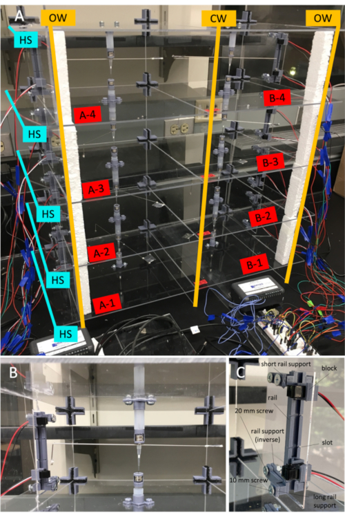
Figure 2: Assembled flight mill. A) Flight mill assembly. Each horizonal shelf (HS) has been inserted into the open slits of the outside vertical walls (OW) and central vertical wall (CW). Moreover, each cell, or 'chamber', is identified with a channel letter (A or B) that corresponds to a data logger and a channel number (1-4) that corresponds to the channel on the specific data logger. B) Flight mill cell assembly with flight mill arm. Magnetic bearings can be raised or lowered by sliding the inner tubes within the outer tubes to adjust the height of the arm. The IR sensors can be also be raised or lowered to align the sensors with the height of the flag on the arm. IR sensors can also be removed from their linear guide rail blocks easily if they need to be replaced or inspected or if the flight mill needs to be transported. Cross brackets provide structural support for each acrylic cell and can be easily inserted and removed. C) Linear guide rail and block assembly in the cell window. All 3D components and respective screws in the cell window are labeled for clearer assembling. Please click here to view a larger version of this figure.

Figure 3: 3D printed designs. Measurements are in mm. A) Linear guide rail. B) Linear guide rail block shaped to hold an IR sensor. C) Screw used as support to replace iron screws. D) Tube support. E) Magnet support. F) Cross bracket used as an acrylic frame aligner and stabilizer. G) Long support and H) short support to keep the linear guide rails in place. Only linear guide rail supports that rest on the outside face of the acrylic wall are shown. Linear guide rail support mirrors are not shown. Please click here to view a larger version of this figure.

Figure 4: Flight mill electrical circuitry. A) Simple diagram of an electric circuit connecting the IR sensors to the data logger. When the flag on the mill arm interrupts the beam emitted by the IR sensor transmitter, the current stops flowing to the IR sensor receiver and the voltage drops to zero. The data logger records all drops in voltage. B) Electrical circuits highlighted. Each yellow box delimits the components of a circuit connected to the breadboard. Multiple electric circuits can be connected to a single breadboard in alternating rows. The size of the solderless breadboard limits how many flight cells can be accommodated. Please click here to view a larger version of this figure.

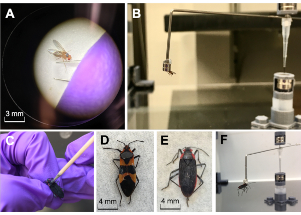
Figure 5: Insects of different sizes magnetically painted and tethered. A) Drosophila melanogaster (common fruit flies) magnetically painted and tethered. Fruit flies are small insects (body length 5 mm; mass = 0.2 mg) that need to first be anesthetized with ice or CO₂ under a microscope before applying the magnetic paint to their thorax. B) Mismatch between insect size and magnet size. The magnet on the flight mill arm should best accommodate the size of the insect. Here the insect's field of vision is obstructed because the magnet is too large. A smaller conical magnet or magnetic strip would solve this mismatch. C-F) Oncopeltus fasciatus (milkweed bugs) and Jadera haematoloma (soapberry bugs) magnetically painted and tethered. Larger bugs (body length > 5 mm; mass > 0.1 g) can be pinched by their legs before applying a coat of paint on their thorax. Please click here to view a larger version of this figure.

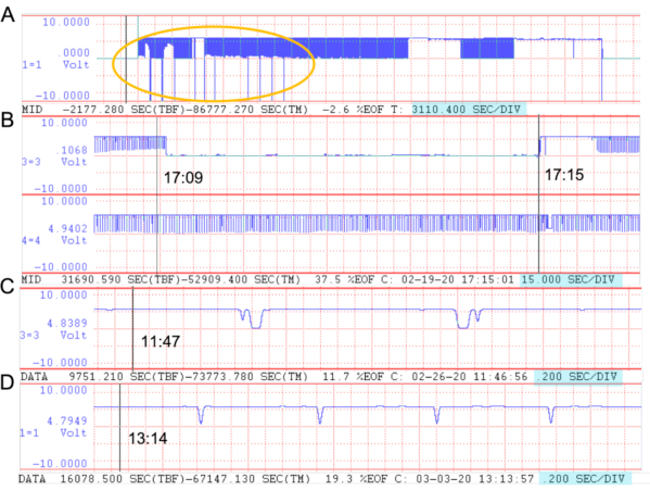
Figure 6: Examples of WDH flight recordings. Voltage troughs represent complete revolutions of the flight mill's arm. The red dotted lines divide the display, and the seconds-per-division (sec/div) of each panel are highlighted in blue. Black vertical lines mark the cursor time. A) Event markers. The sec/div was changed from 0.2 sec/div to its max, allowing the entire waveform to be drawn across the screen. All event markers taken across all channels will only be visible in the first channel as lines that run from the max voltage to the bottom of the channel field window. All event makers for this recording set are within the yellow oval. B) Signal loss. In another recording set, the sec/div was changed from 0.2 sec/div to 15 sec/div to help visualize a recorded signal lost from 17:09 to 17:15 in channel 3. All other channels such as channel 4 continued to function properly. C) Double troughs and mirror troughs. Double troughs are when the voltage dips, rises, and then quickly dips and rises again to create what appears to be two merged troughs in one beam-breaking event. The double troughs also mirror one another, which suggests that the flag moved back and forth between the sensor, which usually happens when an insect stops flying. The Python scripts correct for each case. D) Voltage noise. Soon after 13:14, small bumps in the voltage can be seen, which suggest voltage noise in the recording. Please click here to view a larger version of this figure.

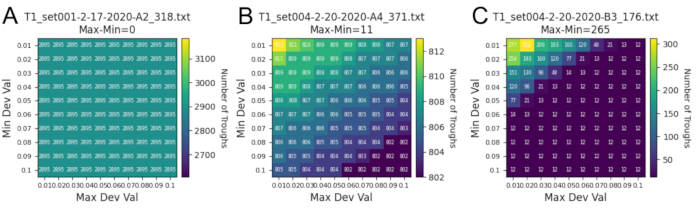
Figure 7: Representative trough diagnostic data from Jadera haematoloma (soapberry bug). Potential noise or overly sensitive troughs are readily recognized in the flight recordings. A) An optimal, robust recording from example individual 318. There was no change in the number of troughs as the minimum and maximum deviation values increased, and so the troughs were robust enough to be identified despite a large standardization interval. B) A sub-optimal, but still robust recording from example individual 371. There is a drop in the number of troughs as the minimum and maximum deviation values increased; however, the drop was minimal (11 troughs). There could be noise and some sensitive troughs but nothing substantial. C) A noisy recording from example individual 176. There is a clear and rapid drop in the number of troughs identified as the minimum and maximum deviation values increased until its number plateaus at 12 troughs. This signals a lot of potential noise or overly sensitive troughs while the 12 troughs remain as robust troughs. Please click here to view a larger version of this figure.

Figure 8: Representative flight data from Jadera haematoloma (soapberry bug). Four categories of flight behavior can be identified in the flight recordings. A) Continuous flight. This individual flew continuously for 1.67 h, beginning at high speeds and then tapering over time into lower speeds. B) Bursting flight. This individual flew only in bursts within the first 30 min of their trial. Bursters can reach high speed but this individual could only retain low speeds. C) Continuous to bursting flight. This individual had maintained continuous flight for 25 min and then tapered off into bursts for the remaining 5 min of their trial. D) Bursting to continuous flight. This individual begun as a burster, reaching high sporadic speeds, and then transitioned into continuous flight for about 4 h. Please click here to view a larger version of this figure.

Figure 9: Representative channel visualization of multiple flight trials within a single recording set. Each color represents an individual soapberry bug at its given channel letter and channel number during its trial. All start times, stop times, and filenames were extracted from each individual's unique flight track .txt file. Please click here to view a larger version of this figure.

Supplemental Figure 1: Kerf key. Kerf is the thickness of the material removed or lost in the process of cutting that material. For a laser cutter, two important factors will determine the width of the kerf: the beam width and the material type. To test and calculate the exact kerf, laser cut the key and fit the 20 mm width key into the slot that it fits most securely. Then, subtract the slot width value from the key width value. For example, a key with a width of 20 mm that fits into a 19.5 mm slot will have a kerf thickness of 0.5 mm. Please click here to download this File.

Supplemental Figure 2: Comparison of low sampling frequencies. A) Relationship between voltage drop and speed by sampling frequency. Each line color and point shape represents a sampling frequency (100 Hz, 75 Hz, 50 Hz, and 25 Hz). Voltage drop is synonymous with the size of the trough. Lines fit second order regressions, which describe the decrease in trough size as speed increases and the following rise in trough size at higher speeds. The shaded bar runs from 0 V to 0.1 V, which marks the voltage range in which noise occurs. Data were collected on cell B-4 using the WinDAQ recording software and with foil flag dimensions 30 mm length by 30 mm width. The flight mill arm was spun rapidly by hand and left to spin until it stopped moving. Sampling frequencies 25 Hz or lower are in danger of misidentifying troughs as noise during standardization and diagnostic tests. Sampling frequencies of 100 Hz or higher are especially robust at recording large troughs for speeds less than 1 m/s. B) Trough sizes of different sampling frequencies seen through the waveform. As the sampling frequencies decrease, their representation on the waveform also shrinks. Please click here to download this File.

Supplemental Figure 3: Flowchart of the functions and data structures of each Python script. An overview of the inputs, functional processes, and outputs of each Python script for the proposed flight mill is summarized and described through examples. Please click here to download this File.

Supplemental 3D Print. Please click here to download this File.

Supplemental Coding Files. Please click here to download this File.

Discussion

The simple, modern flight mill provides a range of advantages for researchers interested in studying tethered insect flight by delivering a reliable and automated design that tests multiple insects efficiently and cost-effectively^13,31,35. Likewise, there is a strong incentive for researchers to adopt fast-emerging technologies and techniques from industry and other scientific fields as a means to build experimental tools to study ecological systems^9,32,33. This protocol takes advantage of two rapidly emerging technologies, the 3D printer and the laser cutter, which are becoming increasingly available in communal makerspaces, in order to enhance the simple, modern flight mill. These enhancements provide a more flexible, adjustable, and collapsible design that accommodates insects of different sizes, minimizes stress placed on the insect, and allows the flight mill to be transported easily to multiple locations or environments. Furthermore, the additional expenses of using the technologies are minimal or even free. However, these technologies can also be a challenge to experiment with if reaching proficiency in using vector graphics editors and 3D image software is not readily available. In turn, the flight mill presented here serves to both encourage researchers to incorporate available emerging technologies in their workflow and to allow researchers to build a customizable, flexible, and effective flight mill without specialized knowledge of electronics, programming, or CAD models.

The strongest aspects of this protocol are the makerspace's technologies that expand a user's flight mill design options, the use of magnetic paint to minimize insect stress, and the automation of flight recordings that processes multiple insects within a single recording. The laser cutter offers precise and exact cutting capabilities that can handle jobs of almost any complexity. The user can modify the acrylic support structure to mount additional 3D prints or purchased items. The 3D printer allows the user to create customizable flight mill components that can bypass costly, pre-made products with narrowly adjustable dimensions. 3D prints not proposed in this paper can also be built, such as landing platforms, supports that can quickly exchange between magnetic bearings and ball bearings, or even a new attachment that tethers an insect. Finally, the use of automated recording software and Python scripts to differentiate multiple flight trials within a single recording makes it possible to study sporadic bouts of flight to very long bouts of flight. However, given how variable flight activity and duration is across species, it is suggested that the user conducts preliminary trials in order to understand the limits and general patterns of a species' flight behavior so as to optimize data collection. The user can also assess the integrity of their recordings using the diagnostic heatmap(s) and can account for any necessary speed corrections in the scripts.

Researchers should also be aware of the flight mill's general constraints. Previous studies have made known and have attempted to remediate the limitations of tethered flight, including a lack of tarsal contact to allow the insect to rest at will^18,31, the absence of energy expended when an insect takes-off³⁴, the additional drag the insect overcomes when pushing the flight mill arm, and the insect needing to compensate for the outward aerodynamic forces experienced due to the centrifugal acceleration of its circular flight track^6,35. Additionally, there continue to be inconsistencies on how to categorize or more precisely quantify the short or 'trivial' bursts insects display, especially when comparing the flight behavior and mechanisms of large migratory insects to those of small insects who exhibit mostly hovering flight^24,36,37. Despite these limitations, there has been significant progress in capturing and categorizing flight behavior within insect species, and researchers have continued to couple the flight mill with other technologies and methods^6,7,8.

The makerspace as a location of creativity, collaboration, and low barriers will further inspire researchers to troubleshoot 3D print design limitations or laser cut more intricate designs. Studies have surveyed the effectiveness of makerspaces not just as iterative product-making spaces but also as places of accelerated learning^10,11,12. Engineering students overall scored higher in design comprehension, design documentation, and model quality when their designs were made using makerspace technology¹¹. Additionally, their model development time dropped by 50%, indicating that makerspace exploration outperformed traditional rote theory and application coursework¹¹. In turn, researchers with little design knowledge will be able to deepen it, and researchers who are also educators can take advantage of this space as a means to increase design organization, craftmanship, and technical dexterity for students. In a discipline like ecology that already makes use of a variety of tools for field and laboratory work, researchers can also develop, share, and standardize novel or enhanced tools. The flight mill proposed in this paper is only the start of what could be an approach to democratizing and rapidly spreading new means of collecting data.

Flight mills have played an important role in enabling researchers to understand the dispersal of insects - an ecological phenomenon still essentially intractable in the field. Future advances in the design and application of the flight mill can be achieved as researchers become more proficient in emerging technologies and the software accompanying those technologies. This could include designing flight mill arm bearings that allow vertical lift or give the insect greater flight orientation flexibility. Additionally, the precision of laser cutters and 3D printers may be necessary for researchers interested in scaling down and calibrating for small insects with mostly hovering capabilities. In turn, the goal of this protocol was to provide an easy entry to these technologies while constructing one of the most common and useful devices in the field of behavioral ecology - the flight mill. If researchers have access to a communal makerspace and are committed to navigating its technologies, the resulting enhancements and improvements of the modern flight mill will lead to creative and collaborative flight mill design and will continue to offer insights into the underlying traits and mechanisms that influence insect species' variations and patterns in movement.

Materials

List of materials used in this article

Name	Company	Catalog Number	Comments
180 Ω Resistor	E-Projects	10EP514180R	Carbon film; stiff 24 gauge lead.
19 Gauge Non-Magnetic Hypodermic Steel Tubing	MicroGroup	304H19RW
2.2 kΩ Resistor	Adafruit	2782	Carbon film; stiff 24 gauge lead.
3D Printer	FlashForge	700355100638
3D Printer Filament	FlashForge	700355100638	Diameter 1.75 mm; 1kg/roll.
3D Printing Slicing Software	FlashPrint	4.4.0
Acrylic Plastic Sheets	Blick Art Supplies	28945-1006
Aluminum Foil	Target	253-01-0860
Breadboard Power Supply	HandsOn Tech	MDU1025	Can take 6.5V to 12V input and can produce 3.3V and 5V.
DI-1100 USB Data Logger	DATAQ Instruments	DI-1100	Has 4 differential armored analog inputs.
Electrical Wires	Striveday	B077HWS5XV	24 gauge solid wire.
Entomological Pins	BioQuip	1208S2	Size 2; diameter 0.45 mm.
Filtered 20 uL Pipette Tip	Fisher Scientific	21-402-550
Hot Glue Gun with Hot Glue	Joann Fabrics	17366956
IR Sensor	Adafruit	2167	This is the 3 mm IR version; works up to 25 cm.
Large Clear Vinyl Tubing	Home Depot	T10007008	Inner diameter 3/8 in; outer diameter 1/2 in; length 20 ft.
Large Magnets	Bunting	EP654	Low-friction N42 neodymium; diameter 0.394 in; length 0.157 in; holding force 4.9 lb.
Laser Cutter	Universal Laser Systems	PLS6.75
M5 Hex Nut	Home Depot	204274112	Thread pitch 0.8 mm; screw length 20 mm; diameter 5 mm.
M5 Long Iron Screws	Home Depot	204283784	Philips pan head; thread pitch 0.8 mm; screw length 20 mm; diameter 5 mm.
M5 Short Iron Screws	Home Depot	203540129	Philips pan head; thread pitch 0.8 mm; screw length 10 mm; diameter 5 mm.
Neoprene Rubber Sheet	Grainger	60DC16	Length 12 in; width 12 in; depth 1/8in.
Online 3D Modeling Software	Autodesk	2019_10_14	Tinkercad.com offers a free account.
Power Adaptor	Adafruit	63	9 VDC 1000mA regulated switching; input voltage DC 3.3V 5V.
Small Clear Vinyl Tubing	Home Depot	T10007005	Inner diameter 1/4 in; outer diameter 3/8 in; 20 ft long.
Small Magnets	Bunting	N42P120060	Low-friction N42 neodymium; diameter 0.120 in; length 0.060 in; holding force 0.5 lb.
Solderless MB-102 Breadboard	Adafruit	239	830 tie points; length 17 cm; width 5.5 cm; input voltage, DC 3.3 V 5 V.
Sophisticated Finishes Iron Metallic Surfacer	Blick Art Supplies	27105-2584
Wire Cutters	Target	84-031W

References

- Krogh, A., Weis-Fogh, T. Roundabout for studying sustained flight of locusts. Journal of Experimental Biology. 29, 211-219 (1952).
- Hocking, B. The intrinsic range and speed of flight of insects. Transactions of the Royal Entomological Society of London. 104 (8), 223(1953).
- Chambers, D. L., O'Connell, T. B. A flight mill for studies with the mexican fruit fly. Annals of the Entomological Society of America. 62 (4), 917-920 (1969).
- Chambers, D. L., Sharp, J. L., Ashley, T. R. Tethered insect flight: A system for automated data processing of behavioral events. Behavior Research Methods & Instrumentation. 8 (4), 352-356 (1976).
- Naranjo, S. E. Assessing insect flight behavior in the laboratory: a primer on flight mill methodology and what can be learned. Annals of the Entomological Society of America. 112 (3), 18(2019).
- Ribak, G., Barkan, S., Soroker, V. The aerodynamics of flight in an insect flight-mill. PLoS ONE. 12 (11), 0186441(2017).
- Pollack, G. S., Martins, R. Flight and hearing: Ultrasound sensitivity differs between flight-capable and flight-incapable morphs of a wing-dimorphic cricket species. The Journal of Experimental Biology. 210, 3160-3164 (2007).
- Koehler, C., Liang, Z., Gaston, Z., Wan, H., Dong, H. 3D reconstruction and analysis of wing deformation in free-flying dragonflies. The Journal of Experimental Biology. 215, 3018-3027 (2012).
- Behm, J. E., Waite, B. R., Hsieh, S. T., Helmus, M. R. Benefits and limitations of three-dimensional printing technology for ecological research. BMC Ecology. 18, 1-13 (2018).
- Sheridan, K. M., et al. Learning in the making: A comparative case study of three makerspaces. Harvard Educational Review. 84, 505-531 (2014).
- Khalifa, S., Brahimi, T. Makerspace: A novel approach to creative learning. Institute of Electrical and Electronics Engineers Xplore. 1, 43-48 (2017).
- Smay, D., Walker, C. Makerspaces: A creative approach to education. Teacher Librarian. 42, 39-43 (2015).
- Attisano, A., Murphy, J. T., Vickers, A., Moore, P. J. A simple flight mill for the study of tethered flight in insects. Journal of Visualized Experiments. 106, e53377(2015).
- Reynolds, D. R., Riley, J. R. Remote-sensing, telemetric and computer-based technologies for investigating insect movement: A of existing and potential techniques. Computers and Electronics in Agriculture. 35 (2-3), 271-307 (2002).
- Davis, M. A. Geographic patterns in the flight ability of a monophagous beetle. Oecologia. 69, 407-412 (1986).
- Taylor, R. A. J., Bauer, L. S., Poland, T. M., Windell, K. N. Flight performance of Agrilus planipennis (Cleoptera: Buprestidae) on a flight mill and in free flight. Journal of Insect Behavior. 23, 128-148 (2010).
- Irvin, N. A., Hoddle, M. S. Assessing the flight capabilities of fed and starved Allograpata obliqua (Diptera: Syrphidae), a natural enemy of Asian citrus psyllid, with computerized flight mills. Florida Entomologist. 103 (1), 139-140 (2020).
- Minter, M., et al. The tethered flight technique as a tool for studying life-history strategies associated with migration in insects. Ecological Entomology. 43 (4), 397-411 (2018).
- Dingle, H., Blakley, N. R., Miller, E. R. Variation in body size and flight performance in milkweed bugs (Oncopeltus). Evolution. 34 (2), 371-385 (1980).
- Martini, X., Hoyte, A., Stelinski, L. L. Abdominal color of the Asian citrus psyllid (Hempitera: Liviidae) is associated with flight capabilities. Annals of the Entomological Society of America. 107 (4), 842-847 (2014).
- Chen, M., et al. Flight capacity of Bactrocera dorsalis (Diptera: Tephritidae) adult females based on flight mill studies and flight muscle ultrastructure. Journal of Insect Science. 15 (1), 141(2015).
- Guo, J., Li, X., Shen, X., Wang, M., Wu, K. Flight performance of Mamestra brassicae Noctuidae) under different biotic and abiotic conditions. Journal of Insect Science. 20 (1), 1-9 (2020).
- Johnson, M. W., Toscano, N. C., Jones, V. P., Bailey, J. B. Modified ultrasonic actograph for monitoring activity of lepidopterous larvae. Proceedings of the Hawaiian Entomological Society. 27, 141-146 (1986).
- Cheng, X., Sun, M. A. Wing-kinematics measurement and aerodynamics in a small insect in hovering flight. Scientific Reports. 6, 25706(2016).
- Holland, J. D. Dispersal kernel determines symmetry of spread and geographical range for an insect. International Journal of Ecology. 2009, 4(2009).
- Frouz, J., Kindlmann, P. Source-sink colonization as a possible strategry of insects living in temporary habitats. PLoS ONE. 10 (6), 1-10 (2015).
- Ventola, C. L. Medical applications for 3D printing: Current and projected uses. Pharmacy & Therapeutics. 39 (10), 704-711 (2014).
- Martí-Campoy, A., et al. Design of a computerized flight mill device to measure the flight potential of different insects. Sensors (Basel). 16 (4), 1-21 (2016).
- Dubois, G. F., Vernon, P., Brustel, H. A flight mill for large beetles such as Osmoderma eremita (Cleoptera: Cetoniidae). Saproxylic Beetles. Their Role and Diversity in European Woodland and Tree Habitats. 14, 219-224 (2009).
- Webster, M. N., Doner, J. P., Wikstrom, V., Lugt, P. Grease degradation in R0F bearing tests. Tribology Transactions. 50 (2), 187-197 (2007).
- Jones, H. B. C., Lim, K. S., Bell, J. R., Hill, J. K., Chapman, J. W. Quantifying interspecific variation in dispersal ability of noctuid moths using an advanced tethered flight technique. Ecology and Evolution. 6 (1), 181-190 (2016).
- Walker, M., Humphries, S. 3D Printing: applications in evolution and ecology. Ecology and Evolution. 9 (7), 4289-4301 (2019).
- Shahrubudin, N., Lee, T. C., Ramlan, R. An overview of 3D printing technology: technological, materials, and applications. Science Direct. 35, 1286-1296 (2019).
- Taylor, R. A. J., Nault, L. R., Styer, W. E., Cheng, Z. B. Computer-monitored, 16-channel flight mill for recording the flight of leafhoppers (Homoptera: Auchenorrhyncha). Journal of the Entomological Society of America. 85 (5), 627-632 (1992).
- Nachtigall, W., Hanauer-Thieser, U., Mörz, M. Flight of the honey bee VII: Metabolic power versus flight speed relation. Journal of Comparative Physiology B. 165, 484-489 (1995).
- Hardie, J. Flight behavior in migrating insects. Journal of Agricultural Entomology. 10 (4), 239-245 (1993).
- Blackmer, J. L., Naranjo, S. E., Williams, L. H. Tethered and untethered flight by Lyrgus Hesperus and Lygus lineolaris (Heteroptera: Miridae). Environmental Entomology. 33 (5), 1389-1400 (2004).
Reprints and Permissions