The study details the methodology of FRET mapping including the selection of labeling sites, choice of dyes, acquisition, and data analysis. This methodology is effective at determining binding sites, conformational changes, and dynamic motions in protein systems and is most useful if performed in conjunction with existing 3-D structural information.
A subscription to JoVE is required to view this content. Sign in or start your free trial.
Method Article
Förster Resonance Energy Transfer Mapping: A New Methodology to Elucidate Global Structural Features
In This Article
Summary
Abstract
Förster resonance energy transfer (FRET) is an established fluorescence-based method used to successfully measure distances in and between biomolecules in vitro as well as within cells. In FRET, the efficiency of energy transfer, measured by changes in fluorescence intensity or lifetime, relates to the distance between two fluorescent molecules or labels. Determination of dynamics and conformational changes from the distances are just some examples of applications of this method to biological systems. Under certain conditions, this methodology can add to and enhance existing X-ray crystal structures by providing information regarding dynamics, flexibility, and adaptation to binding surfaces. We describe the use of FRET and associated distance determinations to elucidate structural properties, through the identification of a binding site or the orientations of dimer subunits. Through judicious choice of labeling sites, and often employment of multiple labeling strategies, we have successfully applied these mapping methods to determine global structural properties in a protein-DNA complex and the SecA-SecYEG protein translocation system. In the SecA-SecYEG system, we have used FRET mapping methods to identify the preprotein-binding site and determine the local conformation of the bound signal sequence region. This study outlines the steps for performing FRET mapping studies, including identification of appropriate labeling sites, discussion of possible labels including non-native amino acid residues, labeling procedures, how to perform measurements, and interpreting the data.
Introduction
For proteins, elucidation of dynamics along with 3-dimensional (3-D) structural knowledge leads to an enhanced understanding of structure-function relationships of biomolecular systems. Structural methods, such as X-ray crystallography and cryogenic electron microscopy, capture a static structure and often require the determination of multiple structures to elucidate aspects of biomolecule binding and dynamics1. This article discusses a solution-based method for mapping global structural elements, such as binding sites or binding interactions, that are potentially more transient and less easily captured by static methods. Strong candidate systems for this methodology are ones in which a 3-D structure has been previously determined by X-ray crystallography, NMR spectroscopy, or other structural methods. In this case, we take advantage of the X-ray crystal structure of the SecA-SecYEG complex, a central player in the protein general secretory pathway, to map the location of a signal peptide binding site using Förster resonance energy transfer (FRET) prior to the transport of the preprotein across the membrane2. Manipulation of the biological system through genetic modifications coupled with our knowledge of the 3-D structure enabled the determination of the conformation of the signal sequence and early mature region immediately prior to insertion into the channel 3.
FRET involves the radiation-less transfer of energy from one molecule (donor) to another (acceptor) in a distance-dependent fashion that is through space4,5. The efficiency of this transfer is monitored through either a decrease in donor or an increase in acceptor fluorescence intensity. The efficiency of energy transfer can be described as
E = R06/(R06 + R6)
in which the R0 value is the distance at which the transfer is 50% efficient6. The technique has previously been described as a molecular ruler and is effective at determining distances in the 2.5-12 nm range, depending on the identity of the donor-acceptor dyes4,7,8,9. The donor fluorescence intensities and lifetimes with or without acceptor allow determination of transfer efficiencies and consequently, distances5,8. Due to the availability of the technology, sensitivity of the method, and ease of use, FRET has also found broad application in such areas as single-molecule fluorescence spectroscopy and confocal microscopy6. The advent of fluorescent proteins such as green fluorescent protein has made the observation of intracellular dynamics and live-cell imaging relatively facile10,11. Many FRET applications such as these are discussed in detail in this virtual issue.
In this study, we particularly focus on the use of FRET measurements to yield distance values to determine structural details. Previously, FRET measurements have been effectively used to determine the conformation of DNA molecules when bound to protein12,13,14, the internal dynamics of proteins, and protein binding interactions15,16,17. The advantages of this method lie in the ability to determine flexible and dynamic structural elements in a solution with relatively low amounts of material. Significantly, this method is particularly effective when used in conjunction with existing structural information and cannot be used as a means of 3-D structure determination. The method provides the best insight and refinement of structure if the work builds on existing structural information often coupled with computational simulation18,19. Here, the use of distances obtained from steady-state and time-resolved FRET measurements is described to map a binding site, the location of which was not known, on an existing crystallographic structure of the SecA-SecYEG complex, major proteins in the general secretory pathway3.
The general secretory pathway, a highly conserved system from prokaryotes to eukaryotes to archaea, mediates the transport of proteins either across or into the membrane to their functional location in the cell. For Gram-negative bacteria, such as E. coli, the organism used in our study, proteins are inserted into or translocated across the inner membrane to the periplasm. The bacterial SecY channel complex (termed the translocon) coordinates with other proteins to translocate the newly synthesized protein, which is directed to its correct location in the cell through a signal sequence typically located at the N-terminus20,21. For proteins bound for the periplasm, the ATPase SecA protein associates with the exit tunnel of the ribosome, and with the preprotein after approximately 100 residues have been translated22. Along with the SecB chaperone protein, it maintains the preprotein in an unfolded state. SecA binds to the SecYEG translocon, and through many cycles of ATP hydrolysis, facilitates protein transport across the membrane23,24.
SecA is a multi-domain protein that exists in cytosolic and membrane-bound forms. A homodimeric protein in the cytosol, SecA consists of a preprotein binding or cross-linking domain25, two nucleotide-binding domains, a helical wing domain, a helical scaffold domain, and the two helix finger (THF)26,27,28,29 (Figure 1). In previous crystallographic studies of the SecA-SecYEG complex, the location of the THF suggested that it was actively involved in protein translocation and subsequent cross-linking experiments with the signal peptide further established the significance of this region in protein translocation30,31. Previous studies, using the FRET mapping methodology, demonstrated that exogenous signal peptides bind to this region of SecA2,32. To fully understand the conformation and location of the signal sequence and early mature region of the preprotein prior to insertion into the SecYEG channel, a protein chimera in which the signal sequence and residues of the early mature region were attached to SecA through a Ser-Gly linker was created (Figure 1). Using this biologically viable construct, it was further demonstrated that the signal sequence and early mature region of the preprotein bind to the THF in a parallel fashion2. Subsequently, the FRET mapping methodology was used to elucidate the conformation and location of the signal sequence and early mature region in the presence of SecYEG as described below3.
Knowledge of the 3-D structure of the SecA-SecYEG complex33,34,35 and the possible location of the binding site allowed us to judiciously place donor-acceptor labels in locations where the intersection of individual FRET distances identifies the binding site location. These FRET mapping measurements revealed that the signal sequence and the early mature region of the preprotein form a hairpin with the tip located at the mouth of the SecYEG channel, demonstrating that the hairpin structure is templated prior to channel insertion.
Access restricted. Please log in or start a trial to view this content.
Protocol
1. Selection of labeling sites
- Identify at least three potential labeling sites to triangulate the putative binding site on the existing protein structures. In this case, SecA, SecYEG, and preprotein attached to SecA through genetic fusion were identified2.
- Choose labeling sites within 25-75 Å of the putative binding site and in relatively static regions of the protein, the distance will determine the specific FRET dye pair to be used36. Locate the labeling sites in protein regions that are relatively distinct from each other, so the sites describe the vertices of a triangle with the putative binding site located in the center (Figure 1A-D).
- Introduce or identify cysteine (Cys) residues at labeling sites of interest in a protein that has no other Cys residues, to improve the labeling efficiency of the specific site37,38.
- Introduce unnatural amino acids, e.g., p-azidophenylalanine for labeling with click chemistry, in order to effectively label one protein at two distinct positions with different dyes39,40.
- Test the Cys mutants for loss of function. Verify the activity of the Cys-less mutant and the unnatural amino acid mutant using an appropriate activity assay. In this case, activity was verified with a growth assay followed by an in vitro malachite green ATPase assay32,41,42
2. Labeling the protein
- Purify the protein or proteins of interest to at least 95% purity for accurate labeling. Purify SecA and SecYEG proteins following protocols detailed in reference3. Ensure that you have at least 5 μg of purified protein for this step, as some protein will be lost during the labeling process.
- Choose two dyes for FRET measurements depending on their R0 value and the predicted distances between labeled sites. Estimate R0 values and observe donor emission and acceptor absorbance overlap using the information from the fluorescent protein database, which also gives spectra for commonly used dyes (https://www.fpbase.org/spectra/)36.
NOTE: R0 is defined as the distance at which the transfer efficiency is 50% for a given dye pair. For mapping experiments, predicted distances should be close to the R0 value of the dye pair to ensure that distances can be measured accurately. - Label the positions identified in step 1.1.1. with the donor-acceptor dye pair.
- Label the protein according to the manufacturer's instructions with particular attention paid to parameters such as optimal protein concentration, temperature, pH, length of time, and buffer for the specific dyes used43,44.
- Prepare the protein at a concentration of 1-2 mg/mL or approximately 10 μM in a 25 mM Tris-HCl (pH 7.5), 25 mM KCl, 1 mM EDTA (TKE) buffer. Dissolve dye in dimethylformamide (DMF) or dimethylsulfoxide (DMSO) to a final concentration of 1 mM. Add the dye dropwise to the solution while stirring to reach a dye: protein molar ratio of 5:1 (50 μM dye: 10 μM protein).
- Allow the reaction to proceed for 4 h at room temperature (RT) in a glass vial with gentle rocking or overnight at 4 °C. Stop the reaction by adding β-mercaptoethanol.
NOTE: If protein is not compatible with Tris buffer, phosphate or HEPES buffers can be used. Maintain pH in the 7.0-7.5 range. If the protein has disulfide bonds, add a reducing agent such as DTT or TCEP prior to labeling. Remove DTT by dialysis or gel filtration before adding dye.
- For accurate FRET measurements remove the free dye with a centrifugal concentrator with an appropriate molecular weight cut-off (MWCO) to let the free dye flow through while retaining the labeled protein.
- Prepare the concentrator membrane by placing ~ 1 mL of water in the upper part of a 3 mL concentrator and then centrifuge the water through the membrane (at least 10 min at 4,300 x g).
- Remove free dye by centrifuging labeled sample in concentrator (20 min at 4,300 x g). Repeat 3-4 times and dispose of flow through.
- Check labeling efficiency of the labeled protein using UV-Vis absorption spectroscopy.
NOTE: FRET measurements require labeling efficiencies of 50% or greater. Lower labeling efficiencies reduce the FRET signal and can lead to inaccuracies in measurement. - Obtain a UV-Vis spectrum of the labeled protein with a range from 250-700 nm to observe both the protein absorption band and the dye maximum absorption band. Measure the absorbance at the absorption peak of dye and at 280 nm for protein.
- Determine the concentration of protein and correct for any contributions from the dye using the correction factor, CF, and the following equations45,46:
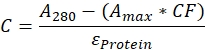
where C is the concentration of the protein (M), A280 is the sample absorbance at 280 nm, Amax is the absorbance at the dye absorption maximum, ε protein is the extinction coefficient for the protein at 280 nm and CF is the correction factor, A'280/A'max, where A'280 is the absorbance at 280 nm and A'max is the absorbance at the peak maximum for the dye only. - Determine labeling efficiency using the following equation:
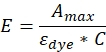
where εdye is the molar extinction coefficient of the dye, C is the concentration of the protein as determined in step 2.4.5, and E is the labeling efficiency. Repeat step 2.4.2 until the labeling efficiency value has plateaued and is less than 100%.
3. Determine the R 0 values
- Measure the R0 values in situ. Prepare two protein samples at the same concentration of total protein, 4 μM, one with the protein labeled with the donor dye only and one with the protein labeled with the acceptor dye only. For SecA, a protein concentration of 4 μM SecA monomer works well for these measurements.
- Prepare sample volumes of 2.5 mL for a 1 cm x 1 cm cuvette, 600 μL for a 5 mm x 5 mm cuvette or 200 μL for a 3 mm x 3 mm cuvette.
- Turn on the fluorometer and open the spectral acquisition and analysis program in the fluorescence software if using a spectrofluorometer. Click on the red M to connect the computer to the instrument (Figure 2A) and choose Emission Spectra.
- Enter scan parameters such as excitation wavelength, the range for emission scan, temperature, and sample changer position using the Collect Experiment menu item (Figure 2B).
- Click on RTC and optimize instrument settings (e.g., spectral slits) by monitoring the fluorescence emission at the peak using an excitation wavelength set at the dye's absorption maximum. For SecA, set the following settings: bandpass as 1 nm; excitation and emission slits as 1 and 1.5 mm respectively, with the temperature at 25 °C and stirring speed at 250 rpm.
NOTE: Do not exceed the counts per second (cps) capacity of the instrument (typically 2 x 10⁶ cps).
- Place the donor labeled protein sample in the sample holder and click Run to generate an emission scan of the protein labeled with the donor dye only (donor only protein) by exciting the sample at the dye absorption maximum (e.g., 488 nm for AF488) and scanning over the emission peak (505-750 nm for donor only SecA protein labeled with AF488).
- Establish a baseline for the scan by extending the scan 25-50 nm past the end of the peak. Measure the quantum yield of the donor-only protein, by performing absorption and fluorescence measurements on samples of different concentrations as described47. Maintain the same slit settings for these measurements.
- Use free donor dye as the reference for the quantum yield. Obtain at least four measurements of the donor-only protein and the free dye at different concentrations for an accurate determination.
- Plot the fluorescence intensity or integrated area versus the absorbance for the donor-only protein and the free dye or reference. Determine the slopes for the donor-only protein (SlopeD) and the reference (SlopeR).
- Quantum yield (Φ) is calculated using the following equation:
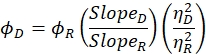
here ΦD is the quantum yield of the donor only protein, ΦR is the quantum yield of the free dye (this can usually be obtained from the manufacturer), SlopeD and SlopeR are the slopes determined in step 3.4.2 for the donor only protein and reference, respectively and ηD and ηR represent the index of refraction of the donor-only protein and the reference-free dye solutions, respectively 47.
- Obtain an absorption spectrum of your acceptor-only protein using a 1 cm pathlength cell. Generate an extinction coefficient spectrum of your acceptor-only protein by dividing the absorption spectrum by the dye concentration.
- Generate the spectral overlap integral, J (λ) using a graphical analysis program. A standard worksheet program (e.g., spreadsheet) can also be used for this process.
- Multiply the fluorescence emission spectrum of the donor-only protein (step 3.4) by the extinction coefficient spectrum of the acceptor-only protein to generate the overlap spectrum.
- Multiply the resultant overlap spectrum by λ4.
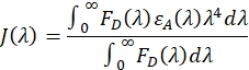
- Determine the area under the curve by integration of the overlap region. The overlap region is defined as the area where the donor emission spectrum multiplied by the acceptor extinction coefficient spectrum yields positive values. The spectral overlap integral is defined as:

where FD (λ) is the emission spectrum of the donor-only protein (obtained in step 3.4) and εA(λ) is the extinction coefficient spectrum of the acceptor-only protein and has units of M-1cm-1 (obtained in step 3.5). The resulting spectral overlap integral should have units of M-1cm-1nm4. - Normalize the spectral overlap integral. Divide the overlap integral by the integrated area of the donor only protein spectrum over the same spectral range:
- Calculate the R0 value in Å using the following equation:

where κ2 is the orientation factor, typically taken as 2/3 for freely rotating dyes, η is the index of refraction and can be approximated as 1.33 for dilute aqueous solutions, QD is the quantum yield of the donor (step 3.4) and J(λ) is the spectral overlap integral as determined in step 3.6.35. NOTE: If the dyes are not freely rotating, corrections can be introduced as described by Ivanov 48 and implemented by Auclair49 and Zhang2,3.
4. Perform FRET spectral measurements
- Prepare donor-only protein, acceptor-only protein, and donor-acceptor protein samples at the same concentration; a concentration of 4 μM is recommended. Use 200 μL of solution, if using a 3 mm x 3 mm cuvette, 600 μL if using a 5 mm x 5 mm cuvette, or 2.5 mL if using a 1 cm x 1 cm cuvette.
- Prepare the donor-acceptor protein sample by using equal molar amounts of the donor only and acceptor only protein.
- Maintain the same amount of labeled sample in control donor only and acceptor only protein samples through the introduction of unlabeled protein in equal molar amount to either the donor only or acceptor only samples. For example, for solutions of the same concentration, each donor-only FRET sample would contain 100 μL of donor-only protein and 100 μL of unlabeled protein for a 200 μL volume.
- Generate fluorescence emission spectra of the donor only, acceptor only, and donor-acceptor samples. Optimize the signal as described in step 3.2. Once optimized maintain the same settings for all of the samples.
- Obtain the donor-only scan as described in step 3.3. Excite the solution at the donor dye absorption maximum and scan over the donor and (expected) acceptor emission peaks.
- Either exchange the sample to the acceptor-only protein or change the sample changer position to the cuvette containing the acceptor-only protein.
- Obtain an emission scan of the protein labeled with acceptor dye only (acceptor only protein) using the same settings as in step 4.2.1. Excite the sample at the donor excitation wavelength.
NOTE: This spectrum provides a correction for the amount of acceptor excited at the donor wavelength (FA in step 5.1.2) - Exchange the sample to the donor-acceptor protein sample or change the sample changer position to the cuvette containing the donor-acceptor labeled protein.
- Obtain an emission scan of the donor-acceptor protein sample using the same settings as in steps 4.2.1 and 4.2.3.
- For all spectra, correct for background fluorescence by subtracting the background counts measured at the end of the scan.
- Measure the donor lifetimes of the donor only and donor-acceptor samples prepared as described in step 4.1.2. Use a time-correlated single-photon counting fluorescence instrument capable of measuring and resolving fluorescent decays in the nanosecond (10-9 s) time range.
NOTE: For FRET dye pairs, match the excitation light source to the absorption maximum of the donor dye.- Turn on the instrument. Open the acquisition software, use the instrument control software for data acquisition with the fluorescence spectrometer.
- For acquisition, select TCSPC Decay, with a time range of 55 ns, a gain of 1 and 4096 channels.
- Obtain an instrument response function (IRF) using a solution of non-dairy creamer or commercial scattering solution and monitor the scattering at 490 nm. Adjust the slit setting and use neutral density filters as needed to maintain a low enough count rate to avoid pulse pile-up5. Click Accept and then Start. This will start the acquisition.
NOTE: A maximum count rate of 4000 cps is used for a 180 kHz repetition rate. - Collect the IRF at 490 nm until the peak channel has a maximum of 20,000 counts. Collect an IRF before and after measuring each fluorescence decay.
- Obtain the fluorescence decays of the donor only and donor-acceptor samples by monitoring the fluorescence emission at the donor emission wavelength, 520 nm.
- Adjust slit settings for a maximum count rate of 4000 cps or less. Slit settings are typically 15-20 nm bandpass for protein samples. Collect the decay until 20,000 counts are obtained in the peak channel.
- Analyze the decay or the fluorescence intensity (I) as a function of time (t) for the fluorescence lifetime (τ). Fit the decay to a sum of exponentials with the following equation:
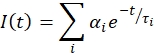
where αI is the preexponential factor of the ith component and τI is the lifetime. The fit is reconvolved with the IRF to match the fluorescence decay. Judge the quality of the fit from the reduced Χ2 parameters.
5. Analysis of FRET data
- Calculate FRET efficiency from the decrease in donor intensity of the donor-acceptor sample relative to the donor only with the following equation.
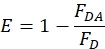
where FDA is the fluorescence intensity of the donor-acceptor sample and FD is the fluorescence intensity of the donor only sample at the peak of the donor fluorescence. Use the integrated areas of the peaks if the data is noisy.- Correct for any differences in labeling between the donor only and donor-acceptor samples. Calculate corrections based on the donor degree of labeling as follows.
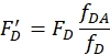
where fDA is the donor labeling efficiency in the donor-acceptor sample and fD is the labeling efficiency in the donor-only sample. - Correct for any contributions of the acceptor fluorescence to the donor-excited spectrum through subtraction of the acceptor-only protein spectrum (step 4.2) from the donor-acceptor protein spectrum.

- Correct for the differences in labeling efficiency of the acceptor only protein relative to the donor-acceptor protein sample yielding the following equation for calculating efficiency:
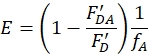
where fA denotes the fractional amount of acceptor labeling. This equation includes all corrections due to dye labeling and acceptor fluorescence. - Calculate FRET distances from the efficiencies using the following equation:
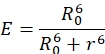
using the R0 value obtained in step 3.6.5. - Calculate FRET efficiency using fluorescence lifetimes of the donor only and donor-acceptor samples measured in step 4.3.3-4.3.5:
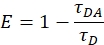
- Use the amplitude-weighted lifetime to calculate FRET efficiencies and compare with steady-state results5.
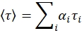
- Calculate the distance as in step 5.1.4 from the efficiencies determined by fluorescence lifetime. Compare steady-state and time-resolved values for FRET efficiencies and distances and ensure that they are within error of each other.
- Correct for any differences in labeling between the donor only and donor-acceptor samples. Calculate corrections based on the donor degree of labeling as follows.
6. Mapping the distances
- Use the calculated distances to map the binding site on the three-dimensional structure. Calculate the distances and errors for all of the dye pairs and locations examined using the equation given in step 5.1.4 and R0 values obtained in step 3.6.5 for each FRET pair.
- Use a 3-D graphical viewing program such as PyMOL50 to map the distances onto the structure (script given in Supplementary File). Commands from the script can be directly entered into the command window with the appropriate distance information.
- Generate a shell for each distance measured and the associated error (Figure 3, Figure 4, Supplementary Figures 1-3).
- Map the position through the intersection of the different shells (Supplementary Figures 1-3). The signal peptide binding site was mapped through the three different locations on SecA and SecYEG and four different locations on the signal peptide (Figure 1).
Access restricted. Please log in or start a trial to view this content.
Results
This study focused on determining the location of the preprotein binding site on SecA prior to insertion of the preprotein into the SecYEG channel. To map the binding site, FRET experiments were performed between different regions of the preprotein and three distinct locations on the SecA and SecYEG proteins (Figure 1A-D). From the distances obtained and three-dimensional structures of SecA, SecYEG, and the preprotein, the location of the preprotein binding ...
Access restricted. Please log in or start a trial to view this content.
Discussion
Through the use of the FRET mapping methodology, we identified the signal sequence binding site on the SecA protein. Importantly, the presence of a 3-D crystal structure of the complex greatly facilitated our study. The strength of this mapping methodology lies in the ability to use an existing structure to identify locations for labeling. This methodology cannot be used to determine a 3-D structure; however, determination of structural elements56, refinement of an existing structure
Access restricted. Please log in or start a trial to view this content.
Disclosures
The authors have nothing to disclose.
Acknowledgements
This work was supported by National Institutes of Health grant R15GM135904 (awarded to IM) and National Institutes of Health Grant GM110552 (awarded to DBO).
Access restricted. Please log in or start a trial to view this content.
Materials
| Name | Company | Catalog Number | Comments |
|---|---|---|---|
| 490 nm LED laser | Horiba | 1684-LED | |
| Alexa Fluor 647 C2 Maleimide//DIBO Alkyne | Life Technologies | A20347 | |
| Agar | Difco | DF0812 | |
| Alexa Fluor 488 C5 Maleimide/DIBO Alkyne | Life Technologies | A10254 | |
| Alexa Fluor 488 DIBO Alkyne | Life Technologies | S10904 | |
| Alexa Fluor 647 DIBO Alkyne | Life Technologies | S10906 | |
| Amicon Ultra4 Centrifugal filter (50kDa MWCO) | Sigma | UFC805008 | |
| Dodecylmaltoside (DDM) | Anatrace | D310 | |
| E. coli alkaline phosphatase signal peptide SP22 | Biomolecules Midwest | N/A | Synthesized custom item |
| extended signal peptide SP41 | Biomolecules Midwest | N/A | Synthesized custom item |
| FluorEssence | Horiba | version 2.4 | spectral acquisition program for Fluoromax4 spectrofluorometer |
| Fluoromax 4 spectrofluorometer | Horiba | N/A | |
| GlobalsWE | Laboratory for Fluorescence Dynamics, University of California, Irvine | spectral analysis program for time-resolved decays | |
| H4AzidoPheOH | BACHEM | 4020250.0001 | |
| LB (Miller) Broth | Fisher Scientific | BP9723 | |
| Ludox HS-40 colloidal silica (40 wt.% suspension in H2O) | Sigma-Aldrich | 420816 | dilution is needed to make a proper scattering solution |
| PTI Felix GX | Horiba | version 4.1.0.4096 | spectral acquisition program for PTI Time Master Instrument |
| PTI Time Master Instrument | Horiba | NA | |
| Pymol Molecular Graphics Program | Schrodinger | version 2.4 | |
| Water bath | Thermo Scientific | NESLAB RTE 10 |
References
- Thompson, M. C., Yeates, T. O., Rodriguez, J. A. Advances in methods for atomic resolution macromolecular structure determination. F1000Research. 9, (2020).
- Zhang, Q., Li, Y., Olson, R., Mukerji, I., Oliver, D. Conserved SecA signal peptide-binding site revealed by engineered protein chimeras and Forester resonance energy transfer. Biochemistry. 55 (9), 1291-1300 (2016).
- Zhang, Q., et al. Alignment of the protein substrate hairpin along the SecA two-helix finger primes protein transport in Escherichia coli. Proceedings of the National Academy of Sciences of the United States of America. 114 (35), 9343-9348 (2017).
- Stryer, L. Fluorescence energy transfer as a spectroscopic ruler. Annual Review of Biochemistry. 47, 819-846 (1978).
- Lakowicz, J. R. Principles of Fluorescence Spectroscopy. , Springer. Boston, MA. (2006).
- Algar, W. R., Hildebrandt, N., Vogel, S. S., Medintz, I. L. FRET as a biomolecular research tool - understanding its potential while avoiding pitfalls. Nature Methods. 16 (9), 815-829 (2019).
- Magde, D., Wong, R., Seybold, P. G. Fluorescence quantum yields and their relation to lifetimes of rhodamine 6G and fluorescein in nine solvents: improved absolute standards for quantum yields. Photochemistry and Photobiology. 75 (4), 327-334 (2002).
- Clegg, R. M. Fluorescence resonance energy transfer and nucleic acids. Methods in Enzymology. 211, 353-388 (1992).
- Scientific, T. F. R0 Values from Some Alexa Fluor Dyes - Table 1.6. , Available from: https://www.thermofisher.com/us/en/home/references/molecular-probes-the-handbook/tables/r0-values-for-some-alexa-fluor-dyes.html (2021).
- Bajar, B. T., Wang, E. S., Zhang, S., Lin, M. Z., Chu, J. A Guide to Fluorescent Protein FRET Pairs. Sensors. 16 (9), Basel, Switzerland. 1488(2016).
- Day, R. N., Davidson, M. W. Fluorescent proteins for FRET microscopy: monitoring protein interactions in living cells. BioEssays : News and Reviews in Molecular, Cellular, and Developmental Biology. 34 (5), 341-350 (2012).
- Lee, S. J., Syed, S., Ha, T. Single-Molecule FRET Analysis of Replicative Helicases. Methods in Molecular Biology. 1805, Clifton, N.J. 233-250 (2018).
- Uhm, H., Hohng, S. Single-Molecule FRET Assay for Studying Cotranscriptional RNA Folding. Methods in Molecular Biology. 2106, 271-282 (2020).
- Globyte, V., Joo, C. Single-molecule FRET studies of Cas9 endonuclease. Methods in Enzymology. 616, 313-335 (2019).
- Qiao, Y., Luo, Y., Long, N., Xing, Y., Tu, J. Single-Molecular Förster Resonance Energy Transfer Measurement on Structures and Interactions of Biomolecules. Micromachines. 12 (5), 492(2021).
- Catipovic, M. A., Bauer, B. W., Loparo, J. J., Rapoport, T. A. Protein translocation by the SecA ATPase occurs by a power-stroke mechanism. The EMBO Journal. 38 (9), 101140(2019).
- Seinen, A. B., Spakman, D., van Oijen, A. M., Driessen, A. J. M. Cellular dynamics of the SecA ATPase at the single molecule level. Scientific Reports. 11 (1), 1433(2021).
- Dimura, M., et al. Quantitative FRET studies and integrative modeling unravel the structure and dynamics of biomolecular systems. Current Opinion in Structural Biology. 40, 163-185 (2016).
- Kalinin, S., et al. A toolkit and benchmark study for FRET-restrained high-precision structural modeling. Nature Methods. 9 (12), 1218-1225 (2012).
- Paetzel, M. Structure and mechanism of Escherichia coli type I signal peptidase. Biochimica et Biophysica Acta. 1843 (8), 1497-1508 (2014).
- Ng, D., Brown, J., Walter, P. Signal sequences specify the targeting route to the endoplasmic reticulum membrane. The Journal of Cell Biology. 134 (2), 269-278 (1996).
- Huber, D., et al. SecA Cotranslationally Interacts with Nascent Substrate Proteins In Vivo. Journal of Bacteriology. 199 (2), 00622(2017).
- Lill, R., et al. SecA protein hydrolyzes ATP and is an essential component of the protein translocation ATPase of Escherichia coli. The EMBO Journal. 8 (3), 961-966 (1989).
- Lill, R., Dowhan, W., Wickner, W. The ATPase activity of SecA is regulated by acidic phospholipids, SecY, and the leader and mature domains of precursor proteins. Cell. 60 (2), 271-280 (1990).
- Kimura, E., Akita, M., Matsuyama, S., Mizushima, S. Determination of a region of SecA that interacts with presecretory proteins in Escherichia coli. The Journal of Biological Chemistry. 266 (10), 6600-6606 (1991).
- Hunt, J. F., et al. Nucleotide control of interdomain interactions in the conformational reaction cycle of SecA. Science. 297 (5589), New York, N.Y. 2018-2026 (2002).
- Sharma, V., et al. Crystal structure of Mycobacterium tuberculosis SecA, a preprotein tranlsocating ATPase. Proceedings of the National Academy of Sciences of the United States of America. 100 (5), 2243-2248 (2003).
- Vassylyev, D., et al. Crystal structure of the translocation ATPase SecA from Thermus thermophilus reveals a parallel, head-to-head dimer. Journal of Molecular Biology. 364 (3), 248-258 (2006).
- Zimmer, J., Li, W., Rapoport, T. A. A novel dimer interface and conformational changes revealed by an X-ray structure of B. subtilis SecA. Journal of Molecular Biology. 364 (3), 259-265 (2006).
- Zimmer, J., Rapoport, T. A. Conformational flexibility and peptide interaction of the translocation ATPase SecA. Journal of Molecular Biology. 394 (4), 606-612 (2009).
- Bauer, B. W., Rapoport, T. A. Mapping polypeptide interactions of the SecA ATPase during translocation. Proceedings of the National Academy of Sciences of the United States of America. 106 (49), 20800-20805 (2009).
- Auclair, S., et al. Mapping of the signal peptide-binding domain of Escherichia coli SecA using Förster resonance energy transfer. Biochemistry. 49 (4), 782-792 (2010).
- Zimmer, J., Nam, Y., Rapoport, T. A. Structure of a complex of the ATPase SecA and the protein-translocation channel. Nature. 455 (7215), 936-943 (2008).
- Li, L., et al. Crystal structure of a substrate-engaged SecY protein-translocation channel. Nature. 531 (7594), 395-399 (2016).
- Ma, C., et al. Structure of the substrate-engaged SecA-SecY protein translocation machine. Nature Communications. 10 (1), 2872(2019).
- Lambert, T. J. FPbase: a community-editable fluorescent protein database. Nature Methods. 16 (4), 277-278 (2019).
- Jilaveanu, L. B., Oliver, D. In vivo membrane topology of Escherichia coli SecA ATPase reveals extensive periplasmic exposure of multiple functionally important domains clustering on one face of SecA. The Journal of Biological Chemistry. 282 (7), 4661-4668 (2007).
- Ramamurthy, V., Oliver, D. Topology of the integral-membrane form of Escherichiacoli SecA protein. The Journal of Biological Chemistry. 272 (37), 23239-23246 (1997).
- Chin, J., et al. Addition of p-Azido-L-phenylalanine to the genetic code of Escherichia coli. Journal of the American Chemical Society. 124 (31), 9026-9027 (2002).
- Deiters, A., et al. Adding amino acids with novel reactivity to the genetic code of Saccharomyces cerevisiae. Journal of the American Chemical Society. 125 (39), 11782-11783 (2003).
- Lanzetta, P. A., Alvarez, L. J., Reinach, P. S., Candia, O. A. An improved assay for nanomole amounts of inorganic phosphate. Analytical Biochemistry. 100 (1), 95-97 (1979).
- Mitchell, C., Oliver, D. B. Two distinct ATP-binding domains are needed to promote protein export by Escherichia coli SecA ATPase. Molecular Microbiology. 10 (3), 483-497 (1993).
- Thiol-reactive Probe Labeling Protocol. Thermo Fischer Scientific. , Available from: https://www.thermofisher.com/us/en/home/references/protocols/cell-and-tissue-analysis/labeling-chemistry-protocols/thiol-reactive-probe-labeling-protocol.html (2021).
- Click Chemistry - Section 3.1. Thermo Fischer Scientific. , Available from: https://www.thermofisher.com/us/en/home/references/molecular-probes-the-handbook/reagents-for-modifying-groups-other-than-thiols-or-amines/click-chemistry.html (2021).
- Correction Factor. AAT Bioquest. , Available from: https://www.aatbio.com/resources/correction-factor/ (2019).
- Calculate dye:protein (F/P) molar ratios. Thermo Fischer Scientific. , Available from: https://tools.thermofischer.com/content/sfs/brochures/TR0031-Calc-FP-rations.pdf (2011).
- A Guide to Recording Fluorescence Quantum Yields. Horiba Scientific. , Available from: https://static.horiba.com/fileadmin/Horiba/Application/Materials/Material_Research/Quantum_Dots/quantumyieldstrad.pdf (2011).
- Ivanov, V., Li, M., Mizuuchi, K. Impact of emission anisotropy on fluorescence stectroscopy and FRET distance measurements. Biophysical Journal. 97 (3), 922-929 (2009).
- Auclair, S., Oliver, D., Mukerji, I. Defining the solution state dimer structure of Escherichia coli SecA using Forster resonance energy transfer. Biochemistry. 52 (14), 2388-2401 (2013).
- The PyMOL Molecular Graphics System, Version 2.4. , Schrodinger, LLC. New York. Available from: https://pymol.org/2/ (2021).
- Musial-Siwek, M., Rusch, S. L., Kendall, D. A. Selective photoaffinity labeling identifies the signal peptide binding domain on SecA. Journal of Molecular Biology. 365 (3), 637-648 (2007).
- Miller, A., Wang, L., Kendall, D. A. Synthetic signal peptides specifically recognize SecA and stimulate ATPase activity in the absence of preprotein. The Journal of Biological Chemistry. 273 (19), 11409-11412 (1998).
- Gelis, I., et al. Structural basis for signal-sequence recognition by the translocase motor SecA as determined by NMR. Cell. 131 (4), 756-769 (2007).
- Erlandson, K. J., et al. A role for the two-helix finger of the SecA ATPase in protein translocation. Nature. 455 (7215), 984-988 (2008).
- Das, S., Oliver, D. Mapping of the SecA-SecY and SecA-SecG interfaces by site-directed in vivo photocross-linking. The Journal of Biological Chemistry. 286 (14), 12371-12380 (2011).
- Wheatley, E. G., Pieniazek, S. N., Vitoc, I., Mukerji, I., Beveridge, D. L. Molecular Dynamics Structure Prediction of a Novel Protein-DNA Complex: Two HU Proteins with a DNA Four-way Junction. Innovations in Biomolecular Modeling and Simulations: Volume 2. , The Royal Society of Chemistry. 111-128 (2012).
- Vitoc, C. I., Mukerji, I. HU binding to a DNA four-way junction probed by Förster resonance energy transfer. Biochemistry. 50 (9), 1432-1441 (2011).
- Hellman, L. M., Fried, M. G. Electrophoretic mobility shift assay (EMSA) for detecting protein-nucleic acid interactions. Nature Protocols. 2 (8), 1849-1861 (2007).
Access restricted. Please log in or start a trial to view this content.
Reprints and Permissions
