Experimental Investigation of Secondary Flow Structures Downstream of a Model Type IV Stent Failure in a 180° Curved Artery Test Section

Summary

Stent implants in stenosed arterial curvatures are prone to "Type IV" failures involving the complete transverse fracture of stents and linear displacement of the fractured parts. We present a protocol for detection of secondary flow (vortical) structures in a curved artery model, downstream of clinically relevant "Type IV" stent failures.

Abstract

The arterial network in the human vasculature comprises of ubiquitously present blood vessels with complex geometries (branches, curvatures and tortuosity). Secondary flow structures are vortical flow patterns that occur in curved arteries due to the combined action of centrifugal forces, adverse pressure gradients and inflow characteristics. Such flow morphologies are greatly affected by pulsatility and multiple harmonics of physiological inflow conditions and vary greatly in size-strength-shape characteristics compared to non-physiological (steady and oscillatory) flows ^{1 - 7}.

Secondary flow structures may ultimately influence the wall shear stress and exposure time of blood-borne particles toward progression of atherosclerosis, restenosis, sensitization of platelets and thrombosis ^{4 - 6, 8 - 13}. Therefore, the ability to detect and characterize these structures under laboratory-controlled conditions is precursor to further clinical investigations.

A common surgical treatment to atherosclerosis is stent implantation, to open up stenosed arteries for unobstructed blood flow. But the concomitant flow perturbations due to stent installations result in multi-scale secondary flow morphologies ^{4 - 6}. Progressively higher order complexities such as asymmetry and loss in coherence can be induced by ensuing stent failures vis-à-vis those under unperturbed flows ⁵. These stent failures have been classified as "Types I-to-IV" based on failure considerations and clinical severity ¹⁴.

This study presents a protocol for the experimental investigation of the complex secondary flow structures due to complete transverse stent fracture and linear displacement of fractured parts ("Type IV") in a curved artery model. The experimental method involves the implementation of particle image velocimetry (2C-2D PIV) techniques with an archetypal carotid artery inflow waveform, a refractive index matched blood-analog working fluid for phase-averaged measurements ^{15 - 18}. Quantitative identification of secondary flow structures was achieved using concepts of flow physics, critical point theory and a novel wavelet transform algorithm applied to experimental PIV data ^{5, 6, 19 - 26}.

Introduction

Secondary flow structures are vortical flow patterns that occur in internal flow geometries with curvatures such as curved pipes and channels. These vortical structures arise due to the combined action of centrifugal forces, adverse pressure gradients and inflow characteristics. In general, secondary flow structures appear in planar cross-sections of curved pipes as symmetric Dean-type vortices under steady inflow and, symmetric Dean- and Lyne-type vortices under oscillatory inflow conditions ^{1 - 3}. Secondary flow morphologies are greatly affected by pulsatility and multiple harmonics of pulsatile, physiological inflow conditions. These structures acquire markedly different size-strength-shape characteristics compared to non-physiological (steady and oscillatory) flows ^{1 - 6}. Atherosclerotic lesion development in arteries is affected by the existence of high frequency shear oscillations in regions experiencing low mean shear ^{27, 28}. Secondary flow structures may influence the progress of diseases such as atherosclerosis and possibly, mediate the endothelial response due to pulsatile blood flow by altering wall shear stresses and exposure times of blood-borne particles.

A common treatment to atherosclerosis, a complication resulting in narrowing of arteries by obstructive lesions, is the implantation of stents. Stent fractures are structural failures of implanted stents that lead to further medical complications such as in-stent restenosis (ISR), stent thrombosis and aneurysm formation ^{9 - 13}. Stent fractures have been categorized into various failure "Types I-to-IV", wherein "Type IV" characterizes the highest clinical severity and is defined as the complete transverse fracture of stent struts along with linear displacements of the stent fragments ¹⁴. The protocol presented in this study describes an experimental method of visualization of secondary flow structures downstream of an idealized "Type IV" stent fracture in a curved artery model.

The suggested protocol has the following four essential features:

Design and fabrication of laboratory-scale stent models: Geometric description of stents can be associated with a set of self-expandable spirals (springs or helices) intertwined using Nitinol (an alloy of nickel and titanium) wires ²⁹. The length of the stent and its strut diameter depend on the length scale of arterial lesions encountered during clinical implantation ⁵. Parametric variation of strut diameter and the rising of the winding (or pitch) leads to stents of various geometric configurations. A summary of stent design parameters chosen for 3D printing are presented in Table 1.

Preparation of a blood analog working fluid matched with kinematic viscosity of blood and refractive index of the test section: Optical access to the curved artery test section is required in order to make non-invasive velocity measurements. Accordingly, a Newtonian blood-mimicking working fluid with the refractive index of the vascular model and ideally, a dynamic viscosity, matching human blood is used to obtain accurate blood flow measurements ^{16 - 18, 30}. The working fluid used in this study was reported by Deutsch et al. (2006), that comprised of 79% saturated aqueous sodium iodide (NaI), 20% pure glycerol, and 1% water (by volume)¹⁶.

Experimental arrangement for the detection of coherent secondary flow structures using a two-component, two-dimensional particle image velocimetry (2C-2D PIV): Experiments were designed to acquire phase-averaged secondary flow velocity data at various planar cross-sectional locations downstream of a combination of straight and curved stent sections embodying an idealized "Type IV" stent fracture ^{5, 6, 9, 14}. The protocol-steps pertaining to the acquisition of secondary flow velocity fields using particle image velocimetry (PIV) technique involves a PIV system that comprises of a laser (light sheet) source, optics to focus and illuminate the regions of flow, a special cross-correlation charge coupled device (CCD-sensor or camera) and tracer particles to be illuminated by the light sheet within a short time interval (Δt; see Table 4) ^{31, 32}.

The steps in the protocol assume the following: First, a calibrated, experimental set-up of a two-component, two-dimensional (2C-2D) PIV system that evaluates images by double-frame, single-exposure recordings. Second, the 2C-2D PIV system calculates the mean displacements of tracer particles by performing cross-correlation between two image frames acquired during each recording. A brief summary of PIV specifications and image acquisition software is presented in the materials and equipment table. Third, all safety precautions needed to operate the laser are followed by trained laboratory personnel according to the guidelines provided by the host institution. The authors suggest Refs. 31 and 32 for a holistic understanding of the implementation, functionality and application of PIV technique in aero-, hydro- and microfluid dynamics, correlation peak detection and displacement estimation, material and density of tracer particles and, measurement noise and accuracy. Also note that the laser and camera can be controlled by the PIV data acquisition computer (Figure 3A) and data processing software.

Data acquisition and post-processing for coherent structure detection: Phase-averaged secondary flow velocity measurements using a 2C-2D PIV were generated using the protocol description that follows. Post-processing of the data involved coherent secondary flow structure detection using the following three methods: continuous wavelet transforms, ^{5, 6, 19 - 24, 26}.

The authors note that the velocity gradient tensor is essentially, a 3 x 3 matrix,
.

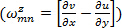
The protocol presents a method of acquiring two-dimensional experimental measurements (from 2C-2D PIV technique). Therefore, full experimental access to the velocity gradient tensor will not be attainable using this method. The velocity gradient tensor for each pixel of the PIV image should be a 2 x 2 matrix, . The z-component vorticity for each pixel is computed using the anti-symmetric part of the velocity gradient tensor . The result will be a 2D array of vorticity that can be visualized in a contour plot. The authors strongly suggest Ref. 25 for an eloquent discussion experimental access to the velocity gradient tensor toward enhancing the knowledge of vorticity dissipation, strain rates and coherent structure detection. Furthermore, the authors do not attempt to explore the inter-relationships between the aforementioned coherent structure detection methods and suggest Ref. 23, 24 for a comprehensive discussion on that subject.

The focus of the steps in the protocol is the quantitative identification of secondary flow (vortical) structures (also known as coherent structures). Three methods of coherent structure detection viz., and wavelet transformed vorticity are applied to velocity field data toward detection of multi-scale, multi-strength occurrences of secondary flow structures downstream of the idealized "Type IV" stent fracture.

The , defines a vortex as a spatial region where the Euclidean norm of the vorticity tensor dominates that of the rate of strain ^{19, 23, 24}.The velocity gradient matrix is decomposed into symmetric (strain rate) and anti-symmetric (rotation) parts. Eigenvalues of strain rate matrix are computed; . Norm of the strain rate is then calculated; . Vorticity is computed from the anti- symmetric part. Enstrophy or square of z-component vorticity, ) is then computed. The is finally computed; . A contour plot of the entire set of with iso-regions of , will indicate secondary flow structures ¹⁹.

The , also known as 'swirling strength' is a vortex identification method performed by critical-point analysis of the local velocity gradient tensor and its corresponding eigenvalues ^{20 - 24}. Eigenvalues of the velocity gradient tensor at each pixel  are computed. The eigenvalues should be of the form, . A contour plot of with iso-regions of will indicate secondary flow structures ^{20 - 22}.

Wavelet transform method utilizes an analyzing function (or wavelet) that has smoothness in physical and spectral spaces, is admissible (or has zero mean) and has a finite ^{5, 6, 26}. By convolving a dilated or contracted wavelet with a 2D vorticity field, wavelet transformed vorticity  field is generated comprising of coherent structures with a wide range of scales and strengths ^{5, 6, 26}. Shannon entropy of the 2D wavelet-transformed vorticity field is computed to estimate the optimal wavelet scale at which all the coherent structures are adequately resolved. This entropy estimation involves a set of probabilities for each pixel such that  , the normalized square modulus of the vorticity associated with the pixel at location m, n ^{5, 6}. The procedural steps are presented graphically in Figure 6. The restrictions placed on the choice of the wavelet are presented in detail in Ref. 26. This protocol step describes the procedure for coherent structure detection using a 2D Ricker wavelet. The justification for the use of this wavelet for vortical pattern matching is presented in Ref. 5, 6 and the pertinent references cited therein.

Protocol

1. Design and Fabrication of Stent Models

Note: The following steps have been followed to create laboratory-scale models of straight and curved stents. The installation of the two stent models will embody a "Type IV" fracture (fragmentation and linear displacement of fractured stent parts).

Note: The authors used Pro/Engineer software at the time of the research for creating CAD models of the stent geometry. The procedure below is generalized and may not include terms generic to the CAD software used. Other CAD packages available can also be used. The steps that follow are applicable for the CAD software that the authors used at the time of the research and have been adapted from the manufacturer's website. For further description of the rapid prototyping machine used by the authors see the Materials List. The parametric equations and initialized values for stent design are presented in Table 1 and Figure 1D and 1E are examples of the straight and curved stent models after rapid prototyping.

1. Create straight stent geometry by defining parametric equations and initializing parameters of the left and right helices in a Cartesian (X-Y-Z) co-ordinate system (Table 1).
   1. Generate a set of 10 equi-spaced left turning helices in a planar circular array about a straight datum line or z-axis, using Eq. 1, 2, 3 and 5 shown in Table 1, with initialized values of number of turns
      (), pitch, stent wire thickness () and nominal diameter of the stent () (Figure 1A and Table 1).
   2. Repeat step 1.1.1 using Eq. 1, 2, 4 and 5 to generate a circular pattern of 10 equispaced left helices (Figure 1A).
   3. Generate straight stent geometry by combining or assembling the left and right turning helices about a common axis (Figure 1A).
2. Create curved stent geometry by defining parametric equations and initializing parameters of the left and right helices in cylindrical (R-β-X) co-ordinate system or about a curved datum line (Table 1). Repeat steps 1.1.1 - 1.1.2 with the previously initialized parameters using Eq. 1, 2, 6 and 7.
   1. Generate a curved stent geometry combining or assembling the left and right turning helices curved about a common axis (R) and subtending an angle at the origin (Figure 1B).
3. Create high-resolution stereo lithography (STL) files from the straight and curved stent CAD models .
   1. Select 'Export > Model' from the 'File menu'. Choose 'STL' option. Set 'chord height' to 0. Set 'Angle control' to 1. Apply 'OK' to create the STL-file. Note: The value of 'Angle Control' regulates the amount of tessellation along surface with small radii and the setting can be between 0 and 1.
4. Fabricate the stent models on a rapid prototyping machine shown in Figure 1C using materials listed in the materials and equipment table.
   1. Start the 3D printing software (see Materials List). Click on 'Insert' to locate the STL-file on the 3D-printer computer and select the desired file. Drag the mouse on the screen to place the 3D rendering of the STL-file on a virtual platform ('Tray') on the screen.
   2. Select appropriate units as 'mm' (Options: 'mm' or 'inches') from the file menu tabs. Select the quality of finished product as 'Matte' (Options: 'Matte' or 'Gloss'). Select 'Tray settings > Validation' tab from the file menus.
   3. Look for the 'Validation succeeded' message to continue to the next step. If validation is unsuccessful repeat steps in 1.3 - 1.4.2 until successful validation is achieved.
   4. Select 'Tray settings > Build' tab from the file menus to send the file to the 3D-printer for fabrication.
      Note: The value of the 'chord height' controls the degree of tessellation of the model surface. It affects the accuracy and file size of the model will be replaced by a minimum value automatically. Small values of chord height leads to less deviation from the actual part geometry with file size tradeoff. Validation check is required to make sure that the part is contiguous and void of any structural anomalies during the fabrication stage.

2. Prepare Kinematic Viscosity– and Refractive Index–matched Blood-analog Fluid

Note: The following procedure will yield approximately 600 ml of blood-analog solution. A summary of the chemical reagents and solvents with relevant properties used in the solution preparation are presented in the Materials List. Relevant material properties, suggested laboratory equipment and the guidelines for volumetric calculations are presented in Tables 2, 3 and 4, respectively.

1. Prepare a saturated solution of Sodium Iodide (NaI).
   1. Pour 500 ml of deionized H₂O into a 2,000 ml beaker. Place the beaker on the magnetic stirrer.
   2. Measure ≈860 g of NaI on a zeroed-weight balance and add 100 g increments into the beaker while stirring and waiting for the current addition to fully dissolve before adding the next. Record the temperature at each addition, since the process of saturation of deionized H₂O with NaI is slightly exothermic. Refrigerate the solution as necessary to maintain it at RT (≈ 25 °C).
   3. Add small NaI increments (≈5-10 g) up to 20 g, until the solution is saturated. Record the mass and temperature of each addition. Remove the beaker with saturated NaI solution from the magnetic stirrer when done.
2. Measure the density of the saturated NaI solution ().
   1. Add 10 ml of saturated NaI solution from step 2.1 to a 50 ml beaker on a zeroed-scale using a syringe (or volumetric pipette), making sure there are no air bubbles. Record mass and the volume added.
   2. Calculate density of each addition using Eq. 8 (see Table 3) . Repeat this step about 4-5 times. Average the densities recorded. Return the solution to the batch of saturated NaI solution prepared in step 2.1.
3. Estimate the total volume of the blood mimicking solution.
   1. Measure the mass of the saturated NaI solution prepared in step 2.1 and calculate its volume () using Eq. 9. Estimate the total volume of the blood mimicking solution () and the partial volumes of glycerol () and deionized water () to be added following Eq. 10, 11 and 12 (see Table 3).
4. Prepare blood-analog solution.
   1. Prepare a blood analog solution comprising of 79% saturated NaI solution, 20% glycerol and 1% deionized water (by volume) through homogenized mixing on a magnetic stirrer.
   2. Place the beaker with the saturated NaI solution on the magnetic stirrer and add glycerol in small increments (), using a syringe (or graduated or volumetric pipette) until the entire volume of glycerol () calculated in step 2.3 is added. For each iteration, record the volume added and wait until the solution is visibly homogenized before the adding the next increment of glycerol.
   3. After complete homogenization of saturated NaI solution and glycerol, add using a syringe (or graduated or volumetric pipette). Continue stirring on the magnetic stirrer until the blood-analog solution is visibly homogenized.
5. Characterize the blood analog fluid at standard ambient temperature and pressure (25 °C, 1 atm).
   1. Measure the kinematic viscosity (ν) using a standard Ubbelohde viscometer or equivalent measuring instrument. Kinematic viscosity can be adjusted by adding small, measured quantities of glycerol using a graduated or volumetric pipette.
   2. Measure the refractive index (n) using a refractometer. Refractive index can be adjusted by adding minute quantities of sodium thiosulfate anhydrous using a spatula.
      Note: The authors report the kinematic viscosity, ν = 3.55 cSt (3.55 x 10^-6 m² sec^-1 ± 2.8%) and the refractive index of the blood analog fluid, n = 1.45 (± 3.4%) ^{5, 6}.

3. Arrange Experiment for Measurement of Secondary Flow Velocity Fields Downstream of a "Type IV" Stent Failure

Note: The 180° curved artery test section comprises of two acrylic blocks glued together, 180° curved channel machined on each block and provision for inlet and outlet pipes as shown in Figures 1F, 3A and 3B. The materials selected for the test section are ensured to have optical accessibility. The authors report the refractive index of material used in the test section as ≈1.4914 ^{5, 6} (See Table 2).

1. Install stents fabricated in step 1 in the curved artery test section made of acrylic to embody an idealized Type IV fracture scenario, entailing a complete transverse fracture of stents and linear displacement of fragmented parts (see Figures 1F, 3A and 3B).
   1. Place the straight stent upstream of the curved artery test section (see Figures 1F and 3B). To ensure that the spacing between the straight and the curved stents is '3 times' the diameter of the tube (D_tube = 12.7 mm), place the 45° curved stent inside the curvature with one end at the inlet to the curved tube (Figure 2B).
2. Assemble the experimental setup by connecting the straight acrylic pipes to the inlet and outlet of the 180° curved artery test section as shown in the schematic overview of the experimental arrangement (Figure 2) on an optical table (Figure 3A).

4. Acquire of Secondary Flow Velocity Fields

Note: The following description in the protocol pertains to the acquisition of secondary flow velocity fields using particle image velocimetry (PIV) technique. Figure 3B (schematic drawing) shows that there four locations (45°, 90°, 135° and 180°) with angular notches to facilitate laser sheet projection and making planar cross-sectional secondary flow velocity. The protocol steps pertain to measurements acquired for the 90° location. If the laser sheet is placed at 45° location, camera is placed at the 135° location to gain optical access for secondary flow measurements at the 45° location.

Note: The procedure below is generalized and may not include terms generic to the image acquisition and post processing software and the instrument control software used (see Materials List). Other image and data acquisition packages available can also be used in the protocol.

1. Turn on the laser using the ON/OFF switches located on the laser power source. Illuminate a small piece of paper to visualize the laser sheet. Adjust the laser sheet thickness(to approximately 2 mm) visually, by turning the laser sheet focusing optics located on the laser source.
2. Place the laser sheet along the 90° measurement region so that the sheet is perpendicular to the optical table. Place the camera near the 0° or 180° location to gain optical access the cross-sectional view illuminated by the laser sheet.
3. Align laser and camera using the image acquisition and post processing software to adjust the field of view of the camera to sufficiently capture the image of the circular cross-section of the curved artery (see Figure 3A) and reducing the particle distortion. Perform the alignment by 'trial and error' by inspecting the software-generated image of the field of view. Switch off the laser using the control switches located on the laser power source and make sure that the camera is turned on with the lens cover removed.
4. Start image acquisition and post processing software on the PIV data acquisition computer and log in as 'expert user'. Create a new project from the file menu, specify a 'Project name' and select 'PIV' option under the 'Type of project'. Select 'New' from the file menu to initialize a new PIV recording session. Select 'Device' under 'Settings' section on image acquisition and post processing software.
5. Navigate to 'Recording' dialogue box on the screen, activate 'Camera 1' check box and select 'Single Frame (T1A)' option. Select laser 'radio button' to be set to ON in the image acquisition and post processing software settings. Activate the external power mode on the laser power source by pressing 'EXT' and 'High power' switches located on the laser power source.
6. Select 'Grab' on the image acquisition and post processing software to start acquiring PIV images to observe on the computer screen. Move camera with slight manual adjustments on the optical table and adjust focus to optimize the location of the camera to maximize the field-of-view, reduce blurriness and image distortion.
7. Select 'Stop' radio button on image acquisition and post processing software settings to cease acquiring PIV data and do not make any further camera adjustments. The alignment procedure is complete at this stage.
   Note: The laser pulses at this stage are controlled by the image acquisition and post processing software and can be further controlled by varying pulsing frequency or 'Exposure' in the software settings. The laser will stop automatically since it is controlled by image acquisition and post processing software. Do not close image acquisition and post processing software as the current project will be used to acquire PIV data in the steps that follow.
8. Acquire images of the secondary flow fields using 2C-2D PIV system by following the steps below to ensure phase-wise PIV data are generated using temporal trigger pulses from the pump instrument control computer that are synchronized with the dual pulse laser and camera.
   Note: The programmable pump is connected to the pump instrument control computer and is controlled by the instrument control software program. The steps that follow involve setting up software control modules on PIV computer using the image acquisition and post processing and pump instrument control computer using instrument control software.
   1. Turn on the programmable pump using the ON/OFF switch located on the pump. Launch the instrument control program on the pump instrument control computer.
   2. Load the text-file that has the values of voltage-time waveform with a reference trigger (t/T = 0), that represents the physiological (carotid artery) flow rate waveform on to the instrument control software maintaining a physiological Womersley number and, maximum Reynolds and Dean numbers (Figure 4A).
   3. Set 'Amplitude' to 1 (Volts), 'DC offset' to 0 (Volts), 'Number of time steps' to 1,000 and 'Time period' to 4 (seconds) on the instrument control software interface screen.
   4. Confirm that the external power mode on the laser power source in Step 4.5, is still activated. Press 'EXT' and 'High power' switches located on the laser power source, if required.
   5. Select 'Device' after clicking 'New Recording' under the 'Settings' section on image acquisition and post processing software. Navigate to the 'Recording' dialogue box on the image acquisition and post processing software (PIV computer), activate 'Camera 1' check box and select 'Double Frame (T1A+T1B)' option to set up the laser to fire in dual pulse mode.
   6. Select 'Timing' option on the 'Recording' dialogue box on the image acquisition and post processing software, select 'Trigger source' and set it to 'External cyclic trigger' to synchronize with trigger-signals from the pump instrument control module. Select 'Aquisit' under the 'Settings' section on the image acquisition and post processing software to start setting up PIV acquisition.
   7. Navigate to the 'Recording sequence' dialogue box on the image acquisition and post processing software. Add a 'Table scan' subcategory under 'Recording sequence' using the appropriate tab provided on the software interface. Populate the table created using 'Edit Table scan', 'Append Scan' and input time values starting with 0 milliseconds and ending with 4,000 milliseconds in intervals of 40 milliseconds. Input Δt-values corresponding to each time entry in table. Press 'Enter' on the keyboard after every value entered.
   8. Navigate to the 'Recording sequence' dialogue box on the image acquisition and post processing software. Add 'Image Acquisition' subcategory under 'Table scan' created in step 4.8.7. Set the 'Number of images' to 200, activate the check box 'Show images while recording' and select 'Start immediately'.
   9. Select 'Device' under the 'Settings' section and confirm that the laser is set to 'ON' with the appropriate power settings. Navigate to 'Laser Control' to confirm. The PIV system is now ready to acquire data.
   10. Select the 'RUN' radio button on instrument control software interface on the pump instrument control computer to supply fluid to the experiment using the inputs provided in step 4.8.2-4.8.3 along with a trigger pulse every 4 seconds.
   11. Select 'Start Recording' for acquiring phase-wise measurements using trigger-signal from the pump instrument control until the predetermined number of planar velocity fields (200, adequate to attain statistical convergence ^{5, 6, 31, 32}) at each time instance set up in the Table scan (see step 4.8.7) at the 90° location is made.
   12. Press 'Stop' on the laser power source once the recording is done. Turn off the pump and camera, and place the camera lens cover. Select 'Stop' radio button on instrument control software interface on the pump instrument control computer.
   13. Visually inspect experimental setup to gage the level of leakage, gather the leaked fluid if necessary, to ensure that all devices have been powered off or can be left on standby, whichever is appropriate. Close the recording session in the image acquisition and post processing software.

5. Detect Coherent Secondary Flow Structures

Note: Use the image acquisition and post processing software and a set of command-line functions (MATLAB-based toolbox, PIVMat 3.01) to import, post-process and analyze 2- component vector fields from the PIV system ^{5, 6, 33}.

1. Create a mask that encompasses the internal flow geometry i.e., the circular, planar cross-sectional area.
   1. Select the project created in step 4.4, that now has PIV data acquired at each instance of time specified in the step 4.8.7. Further, select any data in the dialogue box containing the entire PIV data ensemble.
   2. Follow the instructions in the "Supplemental Code File - creating a mask".
2. Create a post processing routine by selecting 'Batch' icon from the file menu in the project window, while some PIV data set is selected by default. A dialogue box with an 'Operation list' will appear that should be populated in the same order as mentioned in the following step.
   1. Follow the instructions in the "Supplemental Code File - creating a post processing routine".
3. Compute phase-averaged and R.M.S secondary flow velocity, and vorticity fields.
   1. Select the operation 'vector statistics: vector field result' from the group 'statistics' and click on 'Parameter' in the dialogue box. Activate 'Average V' and 'RMS V' check boxes under the 'Vector fields' section. Select the operation 'rot-z Eyx - Exy' from the group 'extract scalar field: rotation and shear' to determine the two-dimensional vorticity in the planar cross-section.
4. Start post processing the entire PIV data and generate phase-averaged quantities of velocity, R.M.S velocity, vorticity and swirling strength with operations created in steps 5.3 and 5.4.
   1. 'Right-click' on any PIV data under the project window, select 'HyperLoop > All sets', and select option 'Add all' under the 'Available Sets:' section to ensure that the entire PIV data ensemble is selected.
   2. Select 'Parameter' from the pull down menu under the 'Filter:' section. Select 'Batch Processing' option under the 'Operation:' section. Click 'Execute' to start 'hyperloop' post processing of the PIV data.
5. Compute swirling strength ) fields to detect secondary flow structures using the image acquisition and post processing software. Select the operation 'swirling strength' from the group 'extract scalar field: rotation and shear'.
   1. Repeat steps 5.4.1-5.4.2 to execute ‘Hyperloop’ post-processing.
6. Detect coherent structures by and continuous wavelet transform on vorticity field by creating user-defined MATLAB functions and using PIVmat 3.01-based MATLAB functions (See "Supplemental Code File - MATLAB codes" for example code).
   1. Generate a 2D array of data from the following equation representing a 2D Ricker wavelet by initializing the scale factor in Eq. 13 to an arbitrary value (See "Supplemental Code File - MATLAB codes").
      
   2. Perform two-dimensional convolution or Fourier multiplication of vorticity data from step 5.4, with 2D Ricker wavelet function (Eq. 13) to generate wavelet transformed vorticity field at the initialized scale factor . (See "Supplemental Code File - MATLAB codes").
   3. Compute the Shannon entropy of the wavelet transformed vorticity field represented by Eq. 14 (See "Supplemental Code File - MATLAB codes").
      
   4. Change the scale factor to  and generate a new 2D array of data representing the 2D Ricker wavelet (Eq. 13) (see Figure 6).
   5. Repeat steps 5.6.1 - 5.6.4, for a large range of scale factors (, see feedback loop in Figure 6.
   6. Create a plot of Shannon entropy vs. wavelet scale factor in step 5.6.5 (see Figure 6). Locate an optimal wavelet scale , usually corresponding to a local minimum in Shannon entropy . Repeat step 5.6.4 at optimum wavelet scale (see Shannon entropy vs wavelet scale plot in Figure 6).
   7. Create a contour plot of the wavelet transformed vorticity  at the wavelet scale factor corresponding to the optimal value of Shannon entropy .

Results

Results presented in Figure 7A-D were generated after post processing secondary flow velocity data (see Figures 5, 6) acquired from 2C-2D PIV system shown in Figure 3A. The inflow condition supplied to the curved artery test section with an idealized "Type IV" stent fracture was the carotid artery waveform shown in Figure 4B. Our previous studies have demonstrated the sensitivity of secondary flow structures to decelerati...

Discussion

The protocol presented in this paper describes the acquisition of high fidelity experimental data using particle image velocimetry technique (PIV) and coherent structure detection methods, viz., continuous wavelet transforms, , suited for identification of vortex and shear-dominated flows. Analysis of experimental data from...

Materials

List of materials used in this article

Name	Company	Catalog Number	Comments
Acrylic tubes and sheet	McMaster-Carr Supply Company		Inlet and outlet pipes and material of the curved artery test section
Object24 Desktop 3D printer	Stratasys		Desktop rapid prototyping machine. http://www.stratasys.com
VeroWhitePlus Opaque material	Stratasys		Building material for Object24 Desktop 3D printer
Fullcure 705	Stratasys		Non-toxic gel-like photopolymer Support material for Object24 Desktop 3D printer
Ubbelohde viscometer	Cole Parmer	YO-98934-12	Toward measurement of kinematic viscosity of the blood-analog fluid
VELP scientifica - ESP stirrer	VELP Scientifica	F206A0179	Magnetic stirrer
Ohaus Scout Pro SP 601	The Lab Depot	SP4001	Weigh scale
Refractometer	Atago	PAL-RI	Toward measurement of refractive index of blood-analog fluid
Beakers, pipettes, syringes and spatula	Sigma-Aldrich	CLS710110,  CLS10031L, CLS71015, CLS71011 Z193216	Toward handling materials required for blood-analog solution preparation
Sodium Iodide	Sigma-Aldrich	383112-2.5KG	Crystalline
Glycerol	Sigma-Aldrich	G5516-1L	Liquid
Deionized Water	-	-	Liquid
Sodium thiosulfate anhydrous	Sigma-Aldrich	72049-250G	Powder
PIV Recording medium	LaVision	Imager Intense 10Hz	PIV Image acquisition CCD camera
PIV Illumination source	New Wave Research	Solo III-15	PIV Laser source, Nd:YAG laser, 532 nm, dual pulse 70 mJ/pulse
PIV Imaging software	LaVision	DaVis 7.2	PIV data acquisition and instrument control
PIV Seeding material	Thermo-scientific	Flouro-Max	Red fluorescent polymer microspheres (≈ 7 µm); Dry dyed polystyrene (DVB) fluorescent microspheres emit bright and distinct colors when illuminated by the light of shorter  wavelengths than the emission wavelength.

References

- Dean, W. R. Note on the motion of a fluid in a curved pipe. Phil Mag. 7, 208-223 (1927).
- Dean, W. R. The streamline motion of a fluid in a curved pipe. Phil Mag. 7, 673-695 (1928).
- Lyne, W. H. Unsteady viscous flow in a curved pipe. J. Fluid. Mech. 45, part 1 13-31 (1970).
- Glenn, A. L., Bulusu, K. V., Shu, F., Plesniak, M. W. Secondary flow structures under stent-induced perturbations for cardiovascular flow in a curved artery model. Int. J. Heat Fluid Fl. 35, 76-83 (2012).
- Bulusu, K. V., Plesniak, M. W. Secondary flow morphologies due to model stent-induced perturbations in a 180° curved tube during systolic deceleration. Exp. Fluids. 54, 1493(2013).
- Bulusu, K. V., Hussain, S., Plesniak, M. W. Determination of secondary flow morphologies by wavelet analysis in a curved artery model with physiological inflow. Exp. Fluids. 55, 1832(2014).
- Womersley, J. R. Method for the calculation of velocity, rate of flow and viscous drag in arteries when the pressure gradient is known. J. Physiol. 127, 553-563 (1955).
- Sheriff, J., Bluestein, D., Girdhar, G., Jesty, J. High-shear stress sensitizes platelets to subsequent low-shear conditions. Ann. Biomed. Eng. 38 (4), 1442-1450 (2010).
- Popma, J. J., Tiroch, K., Almonacid, A., Cohen, S., Kandzari, D. E., Leon, M. B. A qualitative and quantitative angiographic analysis of stent fracture late following sirolimus-eluting stent implantation. Am. J. Cardiol. 103 (7), 923-929 (2009).
- Kim, S. H., et al. A fractured sirolimus-eluting stent with a coronary aneurysm. Ann. Thorac. Surg. 88, 664-665 (2009).
- Adlakha, S., et al. Stent fracture in the coronary and peripheral arteries. J. Interv. Cardiol. 23 (4), 411-419 (2010).
- Alexopoulos, D., Xanthopoulou, I. Coronary stent fracture: How frequent it is? Does it matter. Hellenic J. Cardiol. 52, 1-5 (2011).
- Nair, R. N., Quadros, K. Coronary stent fracture: A review of the literature. Cardiac. Cath. Lab Director. 1, 32-38 (2011).
- Jaff, M., Dake, M., Popma, J., Ansel, G., Yoder, T. Standardized evaluation and reporting of stent fractures in clinical trials of noncoronary devices. Catheter Cardiovasc. Interv. 70, 460-462 (2007).
- Holdsworth, D., Norley, C. J., Frayne, R., Steinman, D. A., Rutt, B. K. Characterization of common carotid artery blood-flow waveforms in normal human subjects. Physiol. Meas. 20 (3), 219-240 (1999).
- Deutsch, S., Tarbell, J. M., Manning, K. B., Rosenberg, G., Fontaine, A. A. Experimental fluid mechanics of pulsatile artificial blood pumps. Annu. Rev. Fluid Mech. 38, 65-86 (2006).
- Yousif, M. Y., Holdsworth, D. W., Poepping, T. L. A blood-mimicking fluid for particle image velocimetry with silicone vascular models. Exp. Fluids. 50, 769-774 (2011).
- Budwig, R. Refractive index matching methods for liquid flow investigations. Exp. Fluids. 17, 350-355 (1994).
- Hunt, J. C. R., Wray, A. A., Moin, P. Eddies, stream, and convergence zones in turbulent flows. Center for Turbulence Research. , Report CTR-S88 (1988).
- Adrian, R. J., Christensen, K. T., Liu, Z. C. Analysis and interpretation of instantaneous turbulent velocity fields. Exp. Fluids. 29, 275-290 (2000).
- Chong, M., Perry, A. E., Cantwell, B. J. A general classification of three-dimensional flow fields. Phys. Fluids A. 2 (5), 765-777 (1990).
- Zhou, J., Adrian, R. J., Balachandar, S., Kendall, T. M. Mechanisms for generating coherent packets of hairpin vortices in channel flow. J. Fluid Mech. 387, 353-396 (1999).
- Haller, G. An objective definition of a vortex. J. Fluid Mech. 525, 1-26 (2005).
- Chakraborty, P., Balachander, S., Adrian, R. J. On the relationships between local vortex identification schemes. J. Fluid Mech. 535, 189-214 (2005).
- Wallace, J. M. Twenty years of experimental and direct numerical simulation access to the velocity gradient tensor: What have we learned about turbulence. Phys. Fluids. 21, 021301(2009).
- Farge, M., Guezennec, Y., Ho, C. M., Meneveau, C. Continuous wavelet analysis of coherent structures. Center for Turbulence Research, Proceedings of the Summer Program. , 331-348 (1990).
- Himburg, H. A., Friedman, M. H. Correspondence of Low Mean Shear and High Harmonic Content in the Porcine Iliac Arteries. ASME J. Biomedical Eng. 128, 852-856 (2006).
- Dai, G., et al. Distinct endothelial phenotypes evoked by arterial waveforms derived from atherosclerosis-susceptible and -resistant regions of human vasculature. PNAS. 101 (41), 14871-14876 (2004).
- Hanus, J., Zahora, J. Measurement and comparison of mechanical properties of nitinol stents. Physica Scripta. 118, 264-267 (2005).
- Segur, J. B., Oberstar, H. E. Viscosity of glycerol and its aqueous solutions. Ind. Eng. Chem. 43, 2117-2120 (1951).
- Adrian, R. J., Westerweel, J. Particle image velocimetry. , Cambridge University Press. NY. (2011).
- Raffel, M., Willert, C. E., Wereley, S. T., Kompenhans, J. Particle image velocimetry - A practical guide, 2nd ed. , Springer. Berlin. (2007).
- Moisy, F. PIVmat 3.01 software. , Laboratoire FAST., University Paris Sud, University Pierre et Marie Curie. CNRS. 91405 Orsay Cedex, France. (2013).
- Ruppert-Felsot, J. E., Praud, O., Sharon, E., Swinney, H. L. Extraction of coherent structures in a rotating turbulent flow experiment. Physical Review E. 72, 016311(2005).
- Bulusu, K. V., Plesniak, M. W. Shannon entropy-based wavelet transform methods for autonomous coherent structure identification in fluid flow field data. Entropy. 17 (10), 6617-6642 (2015).
Access restricted. Please log in or start a trial to view this content.
Reprints and Permissions