Measurements of Waves in a Wind-wave Tank Under Steady and Time-varying Wind Forcing

Summary

This manuscript describes a fully computer-controlled procedure that allows obtaining reliable statistical parameters from experiments of water waves excited by steady and unsteady wind forcing in a small-scale facility.

Abstract

This manuscript describes an experimental procedure that allows obtaining diverse quantitative information on temporal and spatial evolution of water waves excited by time-dependent and steady wind forcing. Capacitance-type wave gauge and Laser Slope Gauge (LSG) are used to measure instantaneous water surface elevation and two components of the instantaneous surface slope at a number of locations along the test section of a wind-wave facility. The computer-controlled blower provides airflow over the water in the tank whose rate can vary in time. In the present experiments, the wind speed in the test section initially increases quickly from rest to the set value. It is then kept constant for the prescribed duration; finally, the airflow is shut down. At the beginning of each experimental run, the water surface is calm and there is no wind. Operation of the blower is initiated simultaneously with the acquisition of data provided by all sensors by a computer; data acquisition continues until the waves in the tank fully decay. Multiple independent runs performed under identical forcing conditions allow determining statistically reliable ensemble-averaged characteristic parameters that quantitatively describe wind-waves' variation in time for the initial development stage as a function of fetch. The procedure also allows characterizing the spatial evolution of the wave field under steady wind forcing, as well as decay of waves in time, once the wind is shut down, as a function of fetch.

Introduction

Since ancient times, it has been well known that waves on water surfaces are excited by wind. The current understanding of the physical mechanisms that govern this process is far from satisfactory. Numerous theories attempting to describe wind-wave generation were proposed over the years^1,2,3,4, however their reliable experimental validation is not yet available. Measurements of random wind-waves in the ocean are extremely challenging due to unpredictable wind that may vary quickly in direction as well as in magnitude. Laboratory experiments have the advantage of controllable conditions that enable prolonged and repeatable measurements.

Under steady wind forcing in the laboratory environment, wind-waves evolve in space. Early laboratory experiments on waves under steady forcing performed decades ago were limited to instantaneous surface elevation measurements^5,6,7,8. More recent studies also employed various optical techniques to measure instantaneous water surface inclination angle, such as LSG^9,10. Those measurements allowed getting some limited qualitative information on the three-dimensional structure of wind-wave fields. When wind forcing is unstable, as it is in field experiments, additional complexity is introduced to the problem of water waves' excitation by wind, since the statistical parameters of the resulting wave field vary not just in space but in time as well. The attempts made so far to describe wave evolution patterns qualitatively and quantitatively under time-dependent forcing were only partially successful^{11,12,13,14,15,16}. The relative contribution of different plausible physical mechanisms that may lead to excitation and growth of waves due to wind action remains largely unknown.

Our experimental facility was designed with the purpose of enabling the accumulation of accurate and diverse statistical information on the variation of wind-wave field characteristics under either steady or unsteady wind forcing. Two major factors facilitated carrying out these detailed studies. First, the modest size of the facility results in relatively short characteristic evolution scales in time and space. Second, the whole experiment is fully controlled by a computer, thus enabling the performance of experimental runs under different experimental conditions automatically and practically without human intervention. These features of the experimental set-up are of crucial importance in performing experiments on waves excited from rest by impulsive wind.

Spatial growth of wind-waves under steady forcing has been studied in our facility for a range of wind velocities¹⁷. Results were compared with growth rate estimates based on the Miles¹⁸ theory as presented by Plant¹⁹. The comparison revealed that the experimental results differ notably from the theoretical predictions. Additional important parameters were also obtained in¹⁷, such as mean pressure drop in the test section, as well as the absolute values and phases of characteristic static pressure fluctuations. The shear stress at the air-water interface is essential for characterization of momentum and energy transfer between wind and waves^17,19. Therefore, detailed measurements of the logarithmic boundary layer and the turbulent fluctuations in the air flow above water waves were performed at numerous fetches and wind velocities²⁰. The values of the friction velocity u_* at the air-water interface determined in this study were used to obtain dimensionless statistical parameters of the wind-waves measured in our facility²¹. These values were compared with the corresponding dimensionless parameters obtained in larger experimental installations and field experiments. It was demonstrated previously²¹ that with proper scaling, the important characteristics of the wind-wave field obtained in our small-scale facility do not differ significantly from the corresponding data accumulated in larger laboratory installations and open sea measurements. These parameters include spatial growth of the representative wave height and wave length, the shape of the frequency spectrum of the surface elevation, as well as the values of higher statistical moments.

The subsequent studies carried out in our facility^22,23 showed that wind waves are essentially random and three-dimensional. To get a better insight into the 3D structure of wind waves, an attempt was made to perform quantitative time-dependent measurements of water surface elevation over an extended area using stereo video imaging²². Due to inadequate computer power available at present and processing algorithms that are not yet sufficiently effective, these attempts proved to be only partially successful. However, it was demonstrated that combined use of a conventional capacitance-type wave gauge and the LSG provides valuable information on the spatial structure of wind waves. Simultaneous application of both those instruments enables independent measurements with high temporal resolution of the instantaneous surface elevation and of the two components of the instantaneous surface slope²³. These measurements allow estimation of both the dominant frequency and dominant wave length of the waves, as well as providing insight into the wave structure in the direction normal to the wind. A pitot tube, which can be moved vertically by a computer-controlled motor, complements the set of sensors and is used for measurements of wind velocity.

All those studies made clear that randomness and three-dimensionality of wind waves result in significant variability of the measured parameters even for steady wind forcing and a single measuring location. Thus, prolonged measurements with duration commensurate with the characteristic time scales of the measured wave field are needed to accumulate sufficient information for extracting reliable statistical quantities. To gain valuable physical insight into the mechanisms governing spatial variation of the wave field, it is imperative to carry out measurements at numerous locations and for as many values of the wind flow rate as possible in the test section. To achieve this goal, it is thus highly desirable to apply an automated experimental procedure.

Experiments on waves excited by unsteady wind forcing introduce an additional level of complexity. In such studies, it is imperative to relate the instantaneous measured parameters to the instantaneous level of the wind speed. Consider experiments on waves excited from rest by a nearly impulsive wind forcing as an important example. In this case, numerous independent measurements are needed of the wind-wave field evolving under the action of wind that varies in time following the same prescribed pattern²⁴. Meaningful statistical parameters, expressed as a function of time elapsed since the initiation of air flow, are then calculated by averaging the data extracted from the accumulated ensemble of independent realizations. This undertaking may involve tens and hundreds of hours of continuous sampling. The total duration of experimental sessions required to accomplish such an ambitious task renders the whole approach unfeasible, unless the experiment is fully automated. No such fully computerized experimental procedure in wind-wave facilities has been developed until recently. That is among the main reasons for the lack of reliable statistical data on wind waves under unsteady forcing.

Since the facility used for the experiment is not constructed from commercially available, off-the-shelf hardware, a brief description of its main parts is provided here.

Figure 1. Schematic (not to scale) view of the experimental facility. 1 - blower; 2 - inflow settling chamber; 3 - outflow settling chamber; 4 - silencer boxes; 5 - test section; with a 6 - beach; 7 - heat exchanger; 8 - honeycomb; 9 - nozzle; 10 - wavemaker; 11 - flap; 12 - instrument carriage; 13 - wave gauge driven by a stepper motor; 14 - Pitot tube driven by a stepper motor. Please click here to view a larger version of this figure.

The experimental facility consists of a closed loop wind tunnel mounted over a wave tank (a schematic view is shown in Figure 1). The test section is 5 m long, 0.4 m wide, and 0.5 m deep. The sidewalls and floor are made of 6 mm thick glass plates and are enclosed within a frame made of aluminum profiles. A 40-cm long flap provides a smooth expansion of the airflow cross-section from the nozzle to the water surface. Wave energy absorbing beach made of porous packing material is located at the far end of the tank. A computer-controlled blower allows attaining mean air flow velocity in the test section up to 15 m/s.

The custom-made capacitance-type 100 mm-long wave gauge is made of anodized tantalum. 0.3 mm wire is mounted on a vertical stage driven by a PC-controlled step motor designed for wave gauge calibration. A Pitot tube with a diameter of 3 mm is used for measuring the dynamic pressure in the central airflow part of the test section.

The LSG, measuring instantaneous 2D water surface slope, is installed on a frame detached from the test section that can be positioned at any location along the tank (Figure 2). LSG consists of four main parts: a laser diode, a Fresnel lens, a diffusive screen, and a Position Sensing Detector (PSD) assembly. The laser diode generates a 650 nm (red), 200 mW focusable laser beam with diameter of about 0.5 mm. The 26.4 cm diameter Fresnel lens with focal length of 22.86 cm directs the incoming laser beam to the 25 x 25 cm² diffusive screen located in the back focal plane of the lens.

Figure 2. Schematic view of the Laser Slope Gauge (LSG). 1 - laser diode; 2 - Fresnel lens; 3 - diffusive screen; 4 - Position Sensor Detector (PSD). Please click here to view a larger version of this figure.

This protocol describes the procedure that allows performing experiments in which numerous parameters characterizing unsteady waves are measured simultaneously under time-dependent wind forcing. The procedure can be adjusted to any desired dependence of wind velocity on time that can be attained in view of the technical limitations of the experimental facility. The present protocol describes specifically experiments in which in every realization, wind starts nearly impulsively over initially calm water. The steady wind forcing then lasts for long enough that the wind-wave field everywhere in the test section attains quasi-steady state. The wind eventually is shut down, again nearly impulsively. At all stages, multiple wave parameters are recorded. The procedure that allows computation of numerous statistically representative ensemble-averaged quantities characterizing the instantaneous local wind-wave field is novel, and was developed in the course of recent experiments carried out in our facility^22,23,24.

Protocol

1. System Preparation

1. Fill the tank with tap water up to a depth of about 20 cm to satisfy deep-water condition; clean the water surface of any contaminants that may affect the surface tension.
2. Position the instrument carriage at the desired fetch.
   1. Mount the Pitot tube and position it at the center of the airflow part of the test section.
   2. Mount the wave gauge on a computer-controlled vertical stage to enable its static calibration.
3. Position the LSG assembly at the desired fetch and at the lateral distance of about 7 cm from the wave gauge to eliminate interference of the wave gauge assembly with the optical path.
   NOTE: The use of an opaque curtain is recommended to prevent the exposure of the PSD to ambient light, as well as to protect the environment from spurious reflections of the laser beam.
   1. Align the laser positioned below the water tank so that the beam is directed vertically, and focus the beam.
   2. Position the fresnel lens within the test section as high as possible above the water surface to minimize the lens's disturbance of the air flow.
   3. Make sure that the deflected laser beam hits the lens in its central part under the extreme wind conditions planned in the experimental session.
   4. Mount the diffusive screen exactly at the focal plane of the lens, then check the horizontal and vertical alignment of both the lens and the screen.
   5. Make sure that any two parallel vertical laser beams hit the diffusive screen exactly at the center when the water surface is still.
      NOTE: This can be tested using two identical lasers positioned at some distance from each other.
   6. Position the PSD making sure that the whole area of the diffusive screen is within the effective area of the detector. Perform focusing of the PSD lens by adjusting the lens settings to the actual distance between the lens and the screen.

2. Calibration and Operation of Sensors

1. Calibration of the wave gauge
   1. Perform wave gauge calibration for each measuring location and each maximum wind velocity expected in the experimental run.
      1. Set the vertical position of the sensor so that the mean water level is approximately in the middle of the sensing wires' length.
      2. Set the blower speed to the desired value, and allow the wind to blow steadily for a sufficiently long time (2 - 3 min).
      3. Using an oscilloscope, manually adjust sensibility, gain, and offset of the wave gauge using the conditioner unit to ensure that the voltage values corresponding to the highest crest and the lowest trough expected in the wave field are within the range of the A/D converter (+/- 10 V).
      4. Shut down the blower for several minutes, until the water's surface becomes completely undisturbed.
      5. Verify that the submerged length is within expected maximum crest and trough values by moving the wave gauge vertically.
      6. Perform automatic calibration of the wave gauge using a custom-made routine in still water submerging the gauge at a number of specified depths and recording the mean voltage output during 5 s for each depth.
      7. Fit a quadratic calibration polynomial to the recorded data to obtain the dependence H(V), where H is the submergence depth (corresponding to the instantaneous surface elevation), as a function of the gauge output voltage V.
      8. Verify visually the quality of the fitted calibration polynomial (Figure 3).

Figure 3. Calibration curve of the wave gauge. Please click here to view a larger version of this figure.

2. Calibration and adjustment of LSG
   1. Verify the performance of the LSG after each displacement of the sensor assembly.
      1. Using an optical wedge prism placed on a horizontal glass sheet, deviate the laser beam with respect to the optical axis simulating a known water surface slope.
      2. Sample the PSD outputs of the deviated laser beam spot at the diffusive screen using an oscilloscope or a custom-built data acquisition program.
      3. Compute the beam deflection angle and the slope from the measured coordinate laser beam spot coordinate; compare the result with the known wedge angle.
      4. Repeat the procedure for several deflection angles using one or more prisms.
         NOTE: Wedge prisms with deflection angles ranging from 2.5° to 17.5° were used; if the test fails due to misalignment of PSD with the diffusive screen, adjust the PSD manually, to correct for misalignment. This procedure is performed manually using a 2D horizontal translation stage and a level and is very time consuming.
   2. Verification of linearity of PSD and calibration procedure
      1. Place an equally spaced grid that has been printed on a transparent sheet on the diffusive screen and orient it so that its axes, x and y, are aligned with the down and cross wind directions, respectively (Figure 4).
         NOTE: The grid facilitates directing the laser beam to the desired locations on the diffusive screen conveniently and accurately either using a set of prisms or moving the laser below the diffusive screen in along-wind and crosswind directions.
      2. Using the set of prisms, deflect the vertical laser beam to obtain multiple radial positions of the laser beam spot on the diffusive screen while maintaining a constant azimuthal angle.
         NOTE: Resolution of 1 cm and maximal radius of 7 cm is used for each of the 9 azimuthal angles.
      3. Move the laser spot to multiple positions in the x-direction, while keeping y coordinate constant, then change the direction of the movement to y, and keep x constant.
         NOTE: Range and resolution used are similar to those from the previous section.
      4. Collect about 50 points on the grid in every calibration.
         NOTE: The laser beam spot coordinates are acquired by PSD and evaluated using a standard two-channel oscilloscope connected to the PSD.
         1. For each direction, use linear fit of the data to yield the calibration coefficients to convert the coordinates of the laser beam on the PSD sensor to the corresponding coordinates on the diffusive screen.
            NOTE: An example of the PSD calibration is plotted in Figure 5 for a set of points taken along the centerline of the test section. The response of the sensor, and thus the calibration coefficients, is nearly identical in all directions when the axes of the diffusive screen and the sensor are aligned properly. The grid facilitates the calibration procedure, allowing an easy determination of the laser slope coordinates on the diffusive screen.

Figure 4. The diffusive screen grid. The grid facilitates directing the laser beam to the desired locations on the diffusive screen conveniently and accurately, either using a set of prisms or moving the laser below the diffusive screen in along-wind and crosswind directions Please click here to view a larger version of this figure.

Figure 5. PSD calibration curve. The figure demonstrates that the translation of the PSD output voltages to coordinates yields adequate results. Please click here to view a larger version of this figure.

3. Experimental Procedure and Data Acquisition

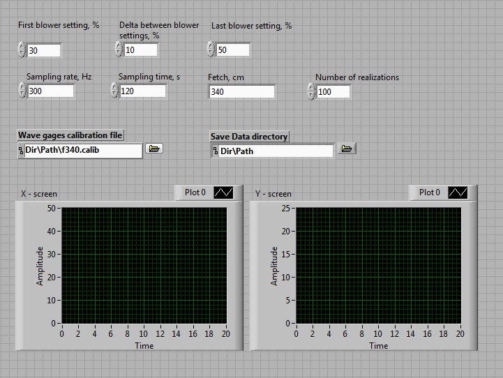
NOTE: See Supplementary Figure 1 for the user interface used in the following steps.

1. Set blower frequency using a custom-built program user interface.
   NOTE: Nearly stepwise increase of the wind velocity over initially undisturbed water surface was applied, followed by a steady airflow rate for a prescribed duration (120 s), and a nearly impulsive shut down of the blower.
2. Determine the number of different steady wind flow rates and the required blower settings.
3. Adjust the pressure transducer settings to the expected range of dynamic pressure variations detected by the Pitot tube.
4. Make sure that at the beginning of each realization, there is no wind and the water surface is undisturbed (mirror smooth). Start data acquisition synchronously with operation of the blower.
5. Record the instantaneous surface elevation, surface slope components in along- and crosswind directions, the Pitot tube output monitoring the mean wind velocity U, and the voltage variation from the blower controller at the prescribed sampling rate (300 Hz/channel were used).
   NOTE: The voltage from wave-gauge acquired by the program is converted automatically to surface elevation using the calibration coefficients from the fit presented in Figure 3.
6. Continue sampling for sufficient time to record the decaying wave field after the shutdown of the blower.
7. Upon completion of the sampling, make sure that the automatic experimental procedure allows for sufficient time (depending on the system) to bring water surface to undisturbed condition prior to the initiation of the next run.
8. Save all the recorded data for subsequent processing.
9. Perform the prescribed number of realizations (usually 100 independent runs were found sufficient).
10. Compute the ensemble-averaged parameters of the recorded data as a function of the time elapsed since the initiation of the blower.
11. Repeat the whole procedure for the next setting of the blower corresponding to the selected target wind velocity in the test section.

Representative Results

The representative ensemble-averaged results are plotted in Figure 6, Figure 7, and Figure 8. The variation of the RMS values of the instantaneous surface elevation <η²>^1/2 that characterizes the amplitude of random wind waves as presented in Figure 6 as a function of time elapsed since initiation of the blower. Results are presented for 3 distances from the wavemaker, x, and for three target wind velocities, U.

For fixed fetch x, the equilibrium quasi-steady state characteristic wave amplitudes increase with the wind velocity U; however, the duration needed to attain the quasi steady value of <η²>^1/2 after initiation of the blower does not seem to depend strongly on U at any given x. The equilibrium values of the characteristic wave amplitudes for a constant target value of the wind forcing U increase with fetch. Note also that variation in the rate of change of <η²>^1/2 is identifiable in each curve plotted in Figure 6, clearly suggesting that distinct stages exist in the wind-waves growth process. The ensemble-averaged RMS values of the downwind and crosswind slope components, <η_x²>^1/2 and <η_y²>^1/2, are plotted in Figure 7 for two fetches and two values of the wind velocity U.

It is evident from the comparison of Figure 6 and Figure 7 that the characteristic time scales of variation of both surface slope components are notably shorter than the corresponding scales of the surface elevation variation. The quasi-steady values of <η_x²>^1/2 and <η_y²>^1/2 are of the same order of magnitude, although the characteristic slopes in the crosswind direction are smaller than the slopes in the along-wind direction. These results indicate that wind-waves are short-crested and three-dimensional. The characteristic slope values in both directions under quasi-steady wind forcing seem to be essentially independent of fetch x, but increase with the wind velocity U. A closer look at the temporal variation of the two slope components for fixed x and U reveals that the initial increase in <η_x²>^1/2 is consistently and notably faster than that of <η_y²>^1/2. Thus, during the very early stage of the growth of the initial ripples that appear on the calm water surface with the activation of wind, they can be seen as approximately two-dimensional. This stage lasts only for a fraction of one second; nevertheless, it is important to emphasize that the essential three-dimensionality of the wave field develops with a certain delay.

The behavior of the wave field after the shutdown of the blower is shown in Figure 8. The waves remaining in the tank decayed fast, effectively vanishing after approximately 1 min.

Figure 6. Temporal variation of the RMS of the surface elevation. The figure demonstrates that the time scales of variation of the characteristic wave height represented by <η²>^1/2 depend on the target wind velocity U and on the fetch x. Please click here to view a larger version of this figure.

Figure 7. Variation with time of the RMS of the downwind/cross-wind surface slope components. The ensemble-averaged RMS values of the downwind and crosswind slope components, <η_x²>^1/2 and <η_y²>^1/2, are plotted here. Please click here to view a larger version of this figure.

Figure 8. Decay of the wind-wave filed after the shutdown of the blower. The ensemble-averaged RMS values of the downwind and crosswind slope components, <η_x²>^1/2 and <η_y²>^1/2, are plotted in Figure 7 for two fetches and two values of the wind velocity U. Please click here to view a larger version of this figure.

Supplementary Figure 1: Custom-built software user-interface for data acquisition. Please click here to download this file.

Discussion

The present experimental protocol is aimed at quantitative characterization of a wave field under unsteady wind forcing that evolves in time and space. Since wind-waves are essentially random and three-dimensional, and thus vary quickly in time and space, records of individual realizations of a growing wind-wave field under time-dependent wind forcing can only provide qualitative estimates of the governing wave parameters. To achieve the goal of this protocol and obtain statistically reliable time- and fetch-dependent wave characteristics, time-resolved ensemble averaging of numerous experimental runs with an identical pattern of wind variation in time has to be applied. Since accumulation of such detailed and extensive information for different target wind velocities and fetches is extremely time consuming, the experimental procedure has to be automated and sufficiently flexible to allow necessary adjustments for different wind forcing conditions. To the best of our knowledge, the experimental procedure described in this manuscript that is capable of providing diverse statistical wave field parameters under variable wind forcing with temporal and spatial resolution was largely unavailable until now.

Note that the duration of experiments required to carry out wind-wave measurements in a laboratory wave tank increases significantly with the size of the facility. This is partially because the duration of the wave growth stage increases with fetch (see Figure 6). The wave lengths and periods also grow with fetch^17,21,23,24, thus for accumulating statistically representative data, the duration of the experiment in each run has to be long compared to the corresponding dominant wave period. Individual realizations at fetches significantly longer than those employed in the present study have thus to be lengthier. Even more important, the longest wavelengths excited by wind in any experimental facility are of the order of the characteristic length of the tank. The residual waves remaining in the tank after the shutdown of the wind in a larger facility thus require longer times for their decay. The interval between the consecutive runs in a bigger wind-wave tank required to return to undisturbed water surface therefore must be considerable longer than the six-minute interval employed in our experiments.

The general approach described above can be applied for a variety of steady and unsteady wind forcing conditions. In this manuscript, the temporal variation of wind forcing was selected with the goal of enabling the accumulation of a sufficient body of data to study unsteady wave field under effectively impulsive wind forcing and shutdown, as well as under steady wind forcing. To this end, care was taken to ensure that the water surface was calm and undisturbed prior to the initiation of each experimental run. In each iteration, the wind was nearly impulsively started by the blower, then the airflow rate remained constant for a sufficiently long time (2 min in the present experiments), after which the blower was shut down. This approach allows studying separately temporally evolving wind-wave fields growing from the initially calm water surface to the quasi-steady state at the given fetch and wind velocity, then the characteristic of waves under steady wind forcing, and finally the decay of waves once wind forcing is abruptly shut down.

The duration of each individual realization in the present study that contains the calm down period thus exceeds 8 min. Therefore, experiments in which data are accumulated for 100 independent runs at a single fetch and target wind velocity last nearly 15 hours (including the duration of the wave gauge calibration procedure). It is obvious that for such an endeavor to be successful, it is imperative that the entire experimental procedure can be carried out automatically, i.e. completely without human intervention.

It thus should be stressed that both the modest size of our facility and the fully automated measuring and calibration procedures were crucial for implementation of the adopted experimental approach. While detailed results on the wind-wave field evolution under unsteady forcing will be presented in the future elsewhere, it is apparent from Figure 6, Figure 7, and Figure 8 that previously unavailable information on fine details of the wind-wave evolution is accumulated in the present study. This information will be used to validate different theoretical models that deal with excitation of waves by wind^1,2,3,4,5,24.

Materials

Name	Company	Catalog Number	Comments
PSD	THORLABS	PDP90A
Laser Diode			any laser pointer ≤ 200 mW
Aspheric Fresnel Lens	EDMUND OPTICS	#46-390	Diameter 10.4'', Focal length 9''
Wave-gauge			custom made
Pressure Transducer	MAMAC SYSTEMS	PR-274-R2-VDC
Signal Conditioner			custom made
Diffusive screen	EDMUND OPTICS	#02-147
Water tank			custome made
A/D card PCI-6221	National Instruments	779066-01
Pitot tube	KIMO Instruments	12971
15° Nom. VIS-NIR Coated, Wedge Prism	EDMUND OPTICS	#47-624
10° Nom. VIS 0° Coated, Wedge Prism	EDMUND OPTICS	#49-444
2.5° Nom. Fused Silica Wedge Prism Uncoated	EDMUND OPTICS	#84-863
4° Nom. Uncoated, Wedge Prism	EDMUND OPTICS	#43-650
5.0° Nom. Fused Silica Wedge Prism Uncoated	EDMUND OPTICS	#84-865
LabView Full Development System	National Instruments	776670-35