Investigating the Relationship between Sea Surface Chlorophyll and Major Features of the South China Sea with Satellite Information

Summary

Sea surface chlorophyll, temperature, sea level height, wind, and front data obtained or derived from satellite observations offer an effective way to characterize the ocean. Presented is a method for the comprehensive study of these data, including overall average, seasonal cycle, and intercorrelation analyses, to fully understand regional dynamics and ecosystems.

Abstract

Satellite observations offer a great approach to investigate the features of major marine parameters, including sea surface chlorophyll (CHL), sea surface temperature (SST), sea surface height (SSH), and factors derived from these parameters (e.g., fronts). This study shows a step-by-step procedure to use satellite observations to describe major parameters and their relationships in seasonal and anomalous fields. This method is illustrated using satellite datasets from 2002–2017 that were used to describe the surface features of the South China Sea (SCS). Due to cloud coverage, monthly averaged data were used in this study. The empirical orthogonal function (EOF) was applied to describe the spatial distribution and temporal variabilities of different factors. The monsoon wind dominates the variability in the basin. Thus, wind from the reanalysis dataset was used to investigate its driving force on different parameters. The seasonal variability in CHL was prominent and significantly correlated with other factors in a majority of the SCS. In winter, a strong northeast monsoon induces a deep mixed layer and high level of chlorophyll throughout the basin. Significant correlation coefficients were found among factors at the seasonal cycle. In summer, high CHL levels were mostly found in the western SCS. Instead of a seasonal dependence, the region was highly dynamic, and factors correlated significantly in anomalous fields such that unusually high CHL levels were associated with abnormally strong winds and intense frontal activities. The study presents a step-by-step procedure to use satellite observations to describe major parameters and their relationships in seasonal and anomalous fields. The method can be applied to other global oceans and will be helpful for understanding marine dynamics.

Introduction

Remote sensing technology offers great datasets with large spatial scales and long periods for describing marine environments. With the increasing spatial resolution of satellites, detailed features are now resolved from the regional scale to a few hundred meters^1,2. An improved understanding of marine dynamics can be achieved with most updated satellite observations³.

By incorporating multiple sensors on a remote sensing platform, a comprehensive description of different parameters is possible. Sea surface temperature (SST) is the basic parameter that has been observed for more than half a century⁴. Recently, observations for sea surface chlorophyll-a (CHL) have become available and can be used to describe marine productivity⁵. Altimetry satellites are used for measuring sea surface height^6,7, which is strongly related to mesoscale eddy activities in the global ocean^8,9. In addition to eddies, frontal activities are also important for impacting regional dynamics and primary production¹⁰.

The major focus of the current study is to find a standard procedure to describe the spatial distribution and temporal variabilities of different ocean factors. In this method, SST, CHL, SSH, and front-data, which are derived from SST gradients, are analyzed to determine patterns. In particular, the CHL is used to represent the productivity of the ocean, and a method is introduced to investigate the relationship between CHL and other ocean parameters. To validate the method, the time period between October 2002 and September 2017 in the South China Sea was used to examine all parameters. The method can be easily used for other regions around the globe to capture major ocean patterns and explore how marine dynamics impact the ecosystem.

The South China Sea (SCS) was designated as the study region because of its relatively high coverage rate of satellite observations. The SCS is abundant in solar radiation; thus, the CHL is mainly determined by the availability of nutrients^11,12. With more nutrients being transported into the euphotic layer, CHL levels can increase¹³. Mixing, induced by wind, can introduce nutrients into the ocean surface and enhance CHL¹⁴. The SCS is uniquely dominated by a monsoon wind system, which determines the dynamics and ecosystem in the region. The monsoon wind is strongest during winter¹⁵. In summer, the winds change direction and the wind speeds are much weaker than those in winter^16,17. The wind intensity can determine the strength of vertical mixing, such that the mixed layer depth (MLD) deepens as the wind increases in winter and becomes shallower as the wind decreases in summer¹⁸. Thus, more nutrients are transported into the euphotic layer during winter when the wind is strong¹⁹ and CHL reaches its highest point of the year^20,21.

In addition to the wind, the MLD can also be determined using other factors, such as SST and sea level anomalies (SLAs), which ultimately impact nutrient content and CHL²². During winter, the weak vertical gradient is associated with low temperatures at the surface²⁰. The corresponding MLD is deep and more nutrients can be transported upward; thus, the CHL in the surface layer is high¹⁷. An increasing variation in CHL levels can be attributed to mesoscale eddies, which induce vertical transport and mixing²³. Upwelling is usually found in cyclonic eddies associated with depressed SLAs^8,9 and elevated CHL concentrations²⁴. Downwelling is usually found in anticyclonic eddies associated with elevated SLAs^8,9 and depressed CHL concentrations²⁴. For other seasons, the MLD becomes shallow, and mixing becomes weak; thus, low CHL can be observed over the majority of the basin²⁵. The seasonal cycles of CHL levels are subsequently predominant for the region²⁶.

In addition to mixing, fronts and their associated coastal upwelling can further modulate the CHL. The front, which is defined as a boundary of different water masses, is important to determine the regional circulation and ecosystem responses²⁷. Frontogenesis is usually associated with coastal upwelling and convergence^28,29, which can induce nutrients and elevate the growth of phytoplankton³⁰. Different algorithms have been developed to automatically identify fronts from satellite observations, including histogram and SST gradient methods. The latter approach is adopted in this study²⁸.

The correlation of time series between CHL and different factors offers great insights for quantifying their relationship. The current study offers a comprehensive description of how to use satellite observations to reveal regional marine dynamics related to productivity. This description can be used as a guide for investigating the surface processes in any part of the ocean. The structure of this article includes a step-by-step protocol, followed by descriptive results in the text and figures. The applicability in addition to the pros and cons of the method are subsequently discussed.

Protocol

1. Dataset acquisition

1. SST and CHL
   1. Download a dataset of satellite observations for SST and CHL from MODIS-Aqua (podaac-tools.jpl.nasa.gov/), where the spatial resolution of both datasets is approximately 4.5 km at daily intervals.
      NOTE: Structure the directories and data following the example scripts folder available in the Supplemental Files. Store the .nc files of the satellite data in the 'Data' folder. Add the path to the NetCDF toolbox in the analysis software (i.e., MATLAB). Select Add with subfolders to enclose the paths of the 'UTILITIES' folder and its subfolders.
   2. Determine the time span. To maintain consistency among different datasets, use the same time span for all parameters. Adjust the time span based on the temporal coverage and use the longest observation period among different datasets. For this protocol, download 15 years of data from October 2002 to September 2017.
   3. Determine the spatial coverage.
      NOTE: The designed study region is between 105°E and 123°E and between 0° and 25°N.
   4. Check preprocessing instructions. Read instructions in the .nc files regarding the preprocessing requirements of the SST and CHL data (e.g., whether scaling is needed).
      NOTE: The downloaded dataset already exclude data over land and within 5 km of the coastline, as well as those contaminated by clouds.
   5. Load SST and CHL data into the analysis software. Type Read_MODIS_SST in the command window to read the SST data. Similarly, type Read_MODIS_CHL in the command window to read the CHL data. Transform the CHL data logarithmically because they have a log-normal distribution³¹.
      NOTE: Loaded variables include SST and CHL in three dimensions, representing meridional location, zonal location, and time in days, respectively. The range of SSTs is between -2 and 44, and the range of CHL is between 0.01 and 20.
2. Sea level anomaly (SLA)
   1. Download daily SLA data with a 25 km spatial resolution from 2002–2017³².
      NOTE: SLAs describe the difference between observed sea surface heights and the mean sea surface height over 20 years (1993−2012) for a corresponding pixel. The SLA data are processed by SSALTO/DUACS and distributed by Archiving, Validation, and Interpretation of Satellite Oceanographic Data (AVISO, https://www.aviso.altimetry.fr).
   2. Load data into the analysis software. Load single-day SLA data by typing Read_SLA in the command window.
      NOTE: The 'Data' folder in the Supplemental Files only includes one sample datum in the script for illustration.
3. Wind speed
   1. Obtain the wind information from an ERA-Interim reanalysis product, which is a global atmospheric reanalysis dataset developed by the European Center for Medium-Range Weather Forecasts (ECMWF)³³. Download wind data for the same period (October 2002–September 2017) to maintain consistency with the CHL and SST data.
      NOTE: The wind dataset has a spatial resolution of approximately 25 km and was interpolated from the original dataset with a spatial resolution of approximately 0.7°.
   2. Load data into the analysis software. Type Read_WindVector in the command window to read the one-month wind data. Calculate the monthly mean by averaging the original data, which is at 6 h intervals.
4. Topography
   1. Download the high-resolution topography data from the National Centers for Environmental Information website (NCEI, https://maps.ngdc.noaa.gov/viewers/wcs-client/). The spatial resolution is ~2 km. Obtain the ETOPO1 data for bedrock in XYZ format for the selected study region.
   2. Load data into the analysis software. Type Read_topography in the command window to load the topography data into the analysis software.

2. Data preprocessing

1. Temporal average
   1. Due to the large cloud coverage in the SST and CHL data, replace the original data with 3-day average data. To do this, after running the Read_MODIS_SST.m and Read_MODIS_CHL.m scripts (step 1.1.5), type Temporal_average in the command window to run the script.
2. Interpolation into the same grid
   1. Because the spatial resolution is not consistent for different datasets, interpolate the SST and CHL data into a spatial grid that is the same as the wind and SLA spatial grid before making comparisons. After running the Temporal_average.m and Read_WindVector.m scripts, type Interpolation_grid in the command window to run the script.
3. Wind stress and wind stress curl
   1. Type Wind_stress_curl in the command window to calculate the wind stress (WS) and wind stress curl (WSC) using the following equations:
      
      
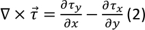
      where is the wind speed vector; is the WS in the same direction as the wind vector; and are the WS in the east and north directions, respectively; is the air density (equal to 1.2 kg/m³); and C is the drag coefficient (a value of 0.0015 is used) under neutral stability conditions³⁴.
4. Monthly averages
   1. Calculate the monthly SST, wind, and SLA time series as 30-day averages in each pixel by typing Monthly_average to run the script. Due to the high cloud coverage rate, use a 60-day average as the monthly time series for CHL, including 30 days before to 30 days after the 15^th day of the month.

3. SST front detection

1. Spatial smoothing
   1. Type Spatial_smoothing to run the script to average the three-day SST data in each pixel.
      NOTE: A large amount of noise was identified in the SST data. Thus, the data were smoothed with a 3 x 3 spatial average. When no data were available in the original 3-day averaged data, the spatial averaged data were set as unavailable.
2. SST gradient
   1. Type SST_gradient to run the script to calculate the zonal and meridional SST gradients (i.e., G_x and G_y, respectively) as the SST difference between the nearest two pixels divided by the corresponding distance via equation (3). Use the obtained gradient vector to calculate the total gradient, G, as a scalar following equation (4).
      
      
3. Local maximum
   1. Identify a front by testing a SST gradient value: label a pixel as a potential frontal pixel if the value is larger than a designated threshold. Only maintain the local maximum pixel in the same direction perpendicular to the gradient direction if there are connected pixels with values larger than the threshold. Here, define the threshold as 0.035 °C/km following former studies^10,28.
      NOTE: The corresponding script ‘Local_maximum.m’ is available in the Supplemental Files.
4. Monthly frontal probability (FP)
   NOTE: The frontal probability (FP) describes the probability of observing a front.
   1. Calculate the FP for a certain time span (in this case, a monthly interval), by typing Monthly_FP to run the script. Divide the occurrence of fronts at each pixel during a time window by the number of days that are free of clouds.

4. Spatial and temporal variability

1. Seasonal cycle
   1. Calculate the seasonal cycles of different factors as the averages of different seasons. Define the seasons as follows: winter is from December to February, spring is from March to May, summer is from June to August, and fall is from September to November.
      NOTE: The seasonal cycle is not shown in this study; the following method is used to explain the spatial and temporal variability instead.
2. Empirical orthogonal function (EOF)
   1. Remove the temporal average and unavailable pixels. Before conducting the EOF, subtract the overall mean at each pixel and exclude the locations where missing observations exceed 20% because of cloud coverage. Load data by typing load('Monthly_data_for_EOF.mat') in the command window.
   2. Apply an EOF to describe the spatial and temporal variabilities of different parameters. Type Empirical_orthogonal_function.m to run the script to calculate the magnitude (Mag), eigenvalues (Eig), and amplitude (Amp) of the EOFs for the dataset (i.e., time series of monthly averaged SST, wind stress, wind stress curl, CHL, and FP).
      NOTE: The function decomposes the monthly time series into different modes, which are composed of spatial and temporal patterns and the variance explained by each mode decreases with increasing mode number.

5. Intercorrelation

1. Correlation at the seasonal scale
   1. Calculate the correlations between two factors using their time series at each pixel by typing Seasonal_correlation to run the script. Because the seasonal cycle is not removed, check the significance of the correlation for all correlations.
2. Correlation of an anomalous field
   1. Calculate the correlations between the monthly CHL anomalies and other factors, such as SST, WS, fronts, and SLAs. Obtain the monthly anomalies (i.e., the deviation from the mean status) by subtracting the overall average for a corresponding month from the monthly time series. Type Anomalous_correlation to run the script and obtain the correlations.

6. Displaying information and calculating relationships

1. Display satellite information.
   1. Type Sat_SCS_Fig3457 to run the script to generate a showcase of satellite information, including SST, CHL, and frontal distributions. Set the current folder as ‘scripts’ where the data ‘Sat_SCS_data.mat’ are located.
      NOTE: Figure 1, Figure 2, Figure 3, and Figure 4 show SST, CHL, fronts, wind, and topography for the selected date as an example.
2. Display the EOF result by typing Sat_SCS_Fig890.m to run the script.
   NOTE: Figure 5, Figure 6, and Figure 7 describe the spatial magnitude, monthly average, and time series of first two modes for CHL, SST, and fronts, respectively.
3. Calculate the relationship between CHL and other factors at seasonal timescales and for anomalous fields by typing Sat_SCS_Fig1112.m to run the script. Obtain the correlation map for seasonal variabilities (Figure 8) and anomalies (Figure 9).

Results

The spatial and temporal patterns of sea surface CHL in the SCS were described using satellite observations. Satellite information for CHL (Figure 1A) and SST (Figure 1B) can be contaminated by cloud coverage, resulting in a large portion of data not being usable. The reanalyzed wind (Figure 1C) and SLA (Figure 1D) data were not impacted by daily clouds. The topography (Figure 1E) had a prominent impact on the spatial distribution of CHL. High CHL was mainly distributed along the coast, where the topography is shallow. Wind was also influenced by orography, and the lee side of mountains was characterized by weak wind; thus, a prominent WSC was identified southwest of the SCS. In contrast, the SLAs did not depend much on topography, and a region of unusually high SLAs was found in the basin of the SCS.

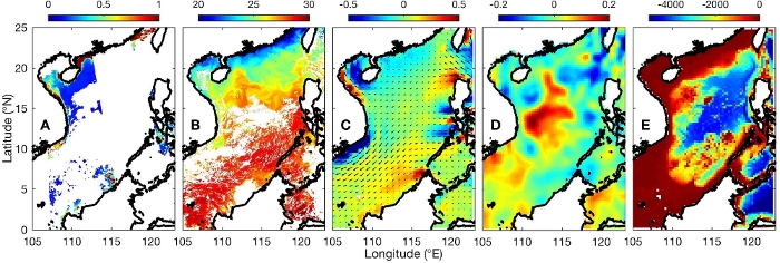
Figure 1: Original observations for major parameters on April 15, 2015.
(A) Sea surface chlorophyll (CHL), (B) sea surface temperature (SST), (C) wind stress curl (WSC, shading) with wind stress (WS, vector), (D) sea surface anomaly, and (E) topography for the ocean basin. Please click here to view a larger version of this figure.

Because of the severe cloud impact on satellite observations, a lot of data were either not available or spatially inconsistent. An effective and efficient method was applied to fill some data gaps and smooth the field. The data were first replaced with a 3-day average at each pixel, which can effectively fill some gaps because clouds vary daily (Figure 2B). A spatial average was further applied at each pixel such that the data were replaced by the mean of surrounding values (3 x 3 pixels). Thus, the spatial inconsistency was greatly reduced (Figure 2C).

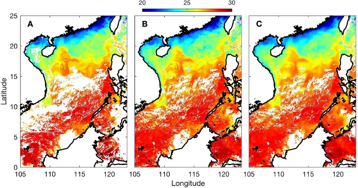
Figure 2: SST for a single day on April 15, 2015.
(A) Original SST from MODIS, (B) three-day averaged SST, and (C) SST after spatial smoothing. Please click here to view a larger version of this figure.

The daily distribution of SST fronts was derived from the SST gradients (Figure 3A). The thresholds applied here effectively captured the location of the front (Figure 3B) and ensured the depiction of the boundaries of entire water masses (Figure 3C). The gradients and fronts were nearly identical because the front were mainly obtained from the gradient.

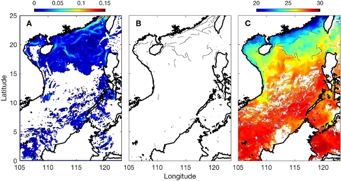
Figure 3: Procedure for front detection derived from SST.
(A) Magnitude of the SST gradient, (B) the distribution of SST fronts in thin black lines, and (C) front distribution based on the corresponding SST gradients. Please click here to view a larger version of this figure.

Due to cloud coverage in the CHL, SST, and front data, the monthly average time series were calculated and applied in this study. A random example is shown in Figure 4 for the month of April 2015. There was no existing gap for any of the parameters. The general patterns for different parameters were highly consistent regarding their spatial variance. For example, CHL was high near the coast and low in the central basin, while the SST was low near the coast and high in the central basin. The monthly average offered comprehensive information to depict regional features. Fronts were mainly distributed along the coast, where the dynamics are complex. A large portion of the basin was free of fronts; thus, the center of the SCS was characterized by a value close to zero (Figure 4E).

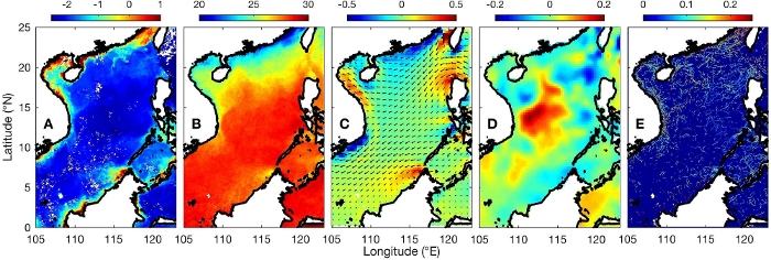
Figure 4: Monthly average for major parameters in April 2015.
(A) CHL (in logarithm scale), (B) SST, (C) WSC (shading) with WS (vector), (D) sea surface anomaly, and (E) frontal probability (FP). Please click here to view a larger version of this figure.

Most surface features were characterized by prominent seasonal variability, which was clearly observed using EOFs. The EOF is a useful mathematic method that is widely used in atmospheric and marine sciences. The method can delineate spatial patterns and temporal signals from time series over spatial domains²⁸. After spatiotemporal decomposition for sea surface features in the SCS, the first two modes are generally needed for describing the spatial and temporal variabilities. The first two EOFs for CHL described 44% and 12% of the total variance, respectively. EOF1 captured a large variance in the northern section of the SCS (Figure 5A). The corresponding monthly average of the time series (Figure 5C) showed that CHL was elevated during the winter and depressed during the summer. The region next to the southwest coast was characterized by weak magnitude, and the corresponding variability was mainly captured by EOF2 (Figure 5B). CHL values were high in the summer and low in the winter. This was mainly out of phase compared with the northern section. The monthly time series for EOFs showed clear seasonal variability, and EOF2 led EOF1 by approximately 4 months (Figure 5E).

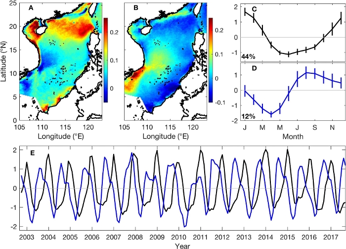
Figure 5: The EOF for CHL.
(A) Magnitude of EOF1, (B) magnitude of EOF2, (C) monthly averaged time series for EOF1, (D) monthly average time series for EOF2, and (E) monthly time series of EOF1 (black) and EOF2 (blue). Please click here to view a larger version of this figure.

The explained variance in the first two EOFs for SST was prominently high, equaling 91% and 5% for EOF1 and EOF2, respectively. It is important to emphasize that the overall average must be removed before conducting EOF; thus, the mean field was excluded. EOF1 dominated the total variance, and its magnitude was largest in the northern SCS and decreased southward (Figure 6A). The corresponding monthly average of the time series (Figure 6C) showed that the SST was elevated during summer and depressed during winter. The southern SCS was characterized by a weak magnitude, attributed to persistent high temperatures at low latitudes. The variability in the southern section was mainly captured by EOF2 (Figure 6B). The corresponding SST was enhanced between March and June, while low values persisted in the remaining months. Prominent warming occurred in 2010 and 2016, where the SST off the coast southwest of the SCS was much higher than that in the other years (Figure 6E). This interannual variability is mainly attributed to El Niño events that reduce the southwest summer monsoon and result in weak upwelling¹². Because seasonal variability is the major focus of the current study, this feature is not discussed further.

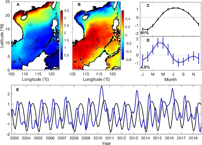
Figure 6: The EOF for SST.
(A) Magnitude of EOF1, (B) magnitude of EOF2, (C) monthly averaged time series for EOF1, (D) monthly averaged time series for EOF2, and (E) monthly time series of EOF1 (black) and EOF2 (blue). Please click here to view a larger version of this figure.

Because of the noisy nature of the gradient, the derived front explained much less of the variance. Indeed, EOF1 and EOF2 of FP only explained 19% and 9% of the total variance, respectively. EOF1 captured the variances in the north and northeast SCS (Figure 7A). The corresponding monthly average of the time series (Figure 7C) showed that in those regions, more FP occurred during winter and less during summer. The phase off the coast southwest of the SCS was the opposite, although the corresponding variability was much less prominent. EOF2 captured the spring enhancement of FP (Figure 7D) in the western SCS (Figure 7B). The monthly time series of EOF1 and EOF2 were characterized by weak interannual variability.

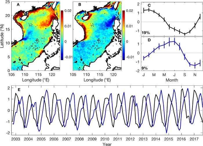
Figure 7: The EOF for FP.
(A) Magnitude of EOF1, (B) magnitude of EOF2, (C) monthly averaged time series for EOF1, (D) monthly averaged time series for EOF2, and (E) monthly time series of EOF1 (black) and EOF2 (blue). Please click here to view a larger version of this figure.

Different factors were investigated for their relationships with CHL (Figure 8). For example, SST can be used to understand the fundamental features of the ocean that can influence the growth rate of phytoplankton and subsequently impact CHL. For the majority of the SCS, there were high correlations between SST and CHL (Figure 8A), and most of the correlations reached more than -0.8. It is important to point out that high correlation does not indicate causation between these two factors. As SST reached its annual maximum in summer, the MLD became shallowest²¹. Nutrients supplied to the euphotic layer were low because vertical mixing was blocked by intensive stratification¹³. As a result, low nutrients limited the growth rate of phytoplankton and resulted in low CHL. In contrast, high CHL occurred in winter when the MLD was deeper, and low SST induced weak stratification³⁵.

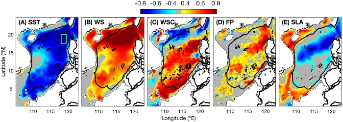
Figure 8: Correlations between CHL and other factors at the seasonal scale.
(A) SST, (B) WS, (C) WSC, (D) FP, and (E) SLA. The gray color indicates that the correlation is nonsignificant. Spatially averaged variables are calculated based on the green box in panel A. Their time series are used to obtain the correlation coefficients in Table 1. This figure has been modified from Yu et al.¹⁷. Please click here to view a larger version of this figure.

Wind-driven mixing can be approximately gauged by WS and was used to describe vertical mixing¹⁸. Large correlation coefficients, with values of approximately 0.8, were identified between the WS and CHL levels north of the SCS (Figure 8B), particularly in the regions with the strongest winter wind located on the northern shelf of the SCS. Weak but significant correlations were found to the south. Correlations between WSC and CHL were significant in the majority of the SCS (Figure 8C), although they showed opposing trends in the north and south. A positive correlation coefficient between CHL and WSC was identified to the south, with negative values were in the north. The correlation in the region between them was not significant. The WS and CHL were found to be strongly correlated in the corresponding region where the winter WS was largest.

Fronts can also induce CHL variability. A large correlation was found in the northeast and southwest of the SCS (Figure 8D). CHL increased as frontal activities became more active³⁶. The SLA showed a significant negative correlation with CHL from the northeast SCS towards the southwest and a positive correlation along the west coast of the SCS (Figure 8E). It is interesting to note that the positive correlations were limited to the region with shallow topography.

To the northeast of the SCS, all correlations were large (Figure 8). Thus, the correlations of monthly time series between CHL and other parameters were calculated using the spatial average in a designated box (Figure 8A), and most of the factors were intercorrelated with significant correlations (top right section of Table 1). Because the seasonal cycle dominated the time series, the correlation was no longer valid after removing the monthly average (bottom left section of Table 1).

	Chl-a	SST	WS	WSC	FP	SLA
Chl-a		-0.8	0.78	0.67	0.74	-0.71
SST	-0.41		-0.47	-0.51	-0.79	0.86
WS	0.32	0.04		0.63	0.51	-0.38
WSC	0	0.08	-0.02		0.52	-0.37
FP	0.21	-0.09	0.03	0.15		-0.74
SLA	-0.25	0.42	0.07	0.13	-0.08

Table 1: Correlation coefficients of the time series among factors, located northeast of the SCS, e.g., SST (sea surface temperature), FP (frontal probability), WSC (wind stress curl) and WS (wind stress), using the box shown in Figure 8A. The monthly averages and anomalies are shown in the top right section and left bottom section, respectively. Numbers in bold and italics indicate that the correlation does not meet the 95% confidence level. The table has been modified from Yu et al.¹⁷.

The correlations in the seasonal cycle were not significant for some regions, such as the southwest of the SCS (Figure 8). The region is dominated by dynamic processes (e.g., upwelling and wind-induced offshore transport) that determine the variability in CHL¹⁷. A significant correlation between CHL and other factors (e.g., SST, WS, fronts, and WSC) was identified in anomalous fields (Figure 9). The anomalies were calculated for the monthly time series by removing the corresponding monthly average. The effective number of degrees of freedom could be increased, but prior studies have shown that it does not impact the underlying relationships among their time series^28,37.

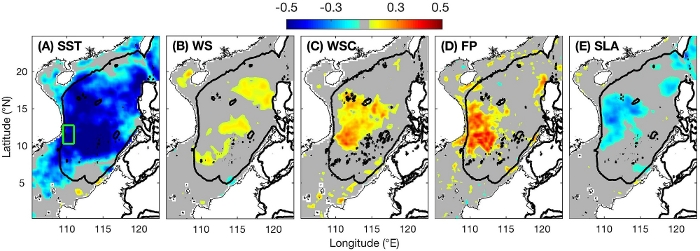
Figure 9: Correlation between CHL and other factors in the anomalous fields.
(A) SST, (B) WS, (C) WSC, (D) FP, and (E) SLA. The gray color indicates that the correlation is nonsignificant. Spatially averaged variables are calculated based on the green box in panel A. The time series are used to obtain the correlation coefficients shown in Table 2. This figure has been modified from Yu et al.¹⁷. Please click here to view a larger version of this figure.

In the anomalous fields, CHL and SST were significantly correlated in the majority of the SCS (Figure 9A). When SSTs were unusually high, CHL became unusually low, and vice versa. Similarly, an unusually high WSC and fronts to the southwest of the SCS induced high levels of CHL, and vice versa (Figure 9C, 9D). In addition, a negative correlation was found between the SLAs and CHL levels (Figure 9E). Different lags were tested, and the correlation only became significant if no lag was employed. Thus, CHL was simultaneously impacted by anomalies in SST, WSC, and fronts, as well as SLA. Their relationship was further investigated using the spatially averaged monthly time series southwest of the SCS, designated as a green box in Figure 9A. The results show that most of the factors were intercorrelated with significant correlations in the anomalous field (bottom left section of Table 2).

	Chl-a	SST	WS	WSC	FP	SLA
Chl-a		-0.15	0.36	0.35	0.26	-0.15
SST	-0.59		-0.48	0.61	0.07	0.17
WS	0.25	-0.24		-0.14	-0.02	0.1
WSC	0.29	-0.1	0.41		0.53	-0.21
FP	0.57	-0.42	0.24	0.29		-0.42
SLA	-0.3	0.54	-0.23	-0.29	-0.47

Table 2: Correlation coefficients of the time series among factors, located southwest of the SCS, e.g., SST (sea surface temperature), FP (frontal probability), WSC (wind stress curl) and WS (wind stress), using the box shown in Figure 9A. The monthly average and anomalies are shown in the top right section and left bottom section, respectively. Numbers in bold and italics indicate that the correlation does not meet the 95% confidence level. The table has been modified from Yu et al.¹⁷.

Supplemental Files. Please click here to download this file.

Discussion

In this study, the major features of marine systems are described using satellite observations. The CHL, which can be used to represent ocean production, is selected as an indicator factor. Factors related to CHL variability were investigated using monthly averaged time series, e.g., SST, WS, WSC, FP and SLA. Three critical steps are described in this study: acquiring satellite data for different parameters, describing their spatial and temporal variabilities via EOF, and determining interrelationships among different factors by calculating correlation coefficients. A detailed procedure showing the identification for daily frontal distribution, which is derived from the SST observations, is included. Two major approaches have been developed for SST front detection: the gradient method^10,38 and the histogram method^39,40. The histogram method is based on a similar range of values for SST, which can be used to divide the water masses into different groups. The pixels with values between different groups representing the pixel in a transitional band are defined as fronts. On the other hand, the gradient method separates several relatively uniform water bodies as pixels with large gradient values. A comparison study was conducted, and they found lower false rates using the histogram method and fewer missed fronts using the gradient method⁴¹. In this study, the gradient-based method³⁸ was adopted following former studies^10,28. The algorithm can avoid front break-up into multiple edge fragments by allowing the magnitude to decrease to a level below a smaller threshold. In addition to the dataset included here, other satellite observations, such as the aerosol index, can also be used with a similar approach.

Most of the procedures can be directly applied in other regions or datasets. Modification may take place to change the threshold of front detection. Because the SST gradient in the SCS is comparable with the Eastern Boundary Current System²⁸, the same thresholds were implemented for the current study. A previous study revealed that the SST gradient from different datasets can vary as much as three times⁴², which makes the method somehow less objective. Substantial studies have investigated frontal activities around the global oceans^28,43. The best approach to validate fronts is to compare them with in situ observations. Yao⁴⁴ described the monthly frontal distribution for the SCS. Their results agreed well with the in situ measurements. The overall gradient should be checked and adjusted since its value may vary depending on the spatial resolution and instruments. In particular, the threshold should be updated when another SST dataset is used. A basic understanding of the regional dynamics is fundamental to understanding frontogenesis^45,46,47. The front detection script can be developed by individual authors based on the description in this paper.

Satellite information offers a comprehensive understanding of surface features, and a results comparison with in situ observations can aid in evaluating credibility. However, satellite observations are limited to the ocean surface, which limits the application for understanding the vertical structure of the water column. In a recent study, satellite observations revealed that the surface CHL increased by 15 times, but the vertical integrated value only increased by 2.5 times⁴⁸. This difference was because the surface value was impacted by the coeffects of phytoplankton growth and shoaling of MLD, resulting in an unrealizable value at the surface. Thus, the surface feature may not offer an accurate description for the entire water column. Additionally, the influence of cloud coverage limits the continuous observations of satellites. Thus, monthly time series are calculated for different factors over the same region and same period. This will guarantee the credibility of calculating the correlations among different factors. However, the short-period events, e.g., typhoons that last for a few days to a week, will not be resolved.

Compared with former studies, the proposed method can offer spatial information at the pixel level, which can help to evaluate the dynamics in a more detailed manner. Some former studies averaged the entire SCS as a single number and obtained a time series. They found that an unusually strong WS and high SST can induce anomalously high CHL¹⁶, which is consistent with the current result. However, the spatial variation in the relationships was not resolved. In this study, the basin-scale correlation between WS and CHL was weak in the anomalous field. A large significant correlation was only identified for certain areas, e.g., in the center of the SCS (Figure 9B). Thus, the current method offers a comprehensive description for investigating spatial variations. Similarly, observations from two Bio-Argo floats were used and revealed that WSC did not correlate with CHL variability²⁰. However, the trajectories of the two floats are only located in certain regions. In this case, it was exactly within the band where the correlation between the CHL level and the WSC was not significant (Figure 8D). The proposed method is very helpful for resolving the spatial dependence among factors, which is a fundamental characteristic of the global ocean.

In summary, the method used here can accurately describe the spatial distribution and temporal variability in ocean surface features using satellite observations. With the increasing resolution of satellite datasets, more detailed features can be identified and investigated, which enables a general understanding of regional features, including CHL, SST, and SSH. The correlation of monthly time series among different factors can aid in understanding their dynamic relationships and potential impact on an ecosystem⁴⁹. Because the correlation can largely vary at different spatial locations, the proposed method offers a detailed and comprehensive description. A similar approach can be applied to any ocean basin worldwide, which will be greatly helpful to improve the understanding of marine dynamics and ecosystems.

Materials

List of materials used in this article

Name	Company	Catalog Number	Comments
Matlab	MathWorks	Matlab R2016	https://www.mathworks.com/products/matlab.html; referred to analysis software in the protocol
Sea surface chlorophyll	NASA	MODIS	mg/mg3 (podaac-tools.jpl.nasa.gov)
Sea surface height	AVISO	AVISO	meter (www.aviso.altimetry.fr)
Sea surface temperature	NASA	MODIS	°C (podaac-tools.jpl.nasa.gov)
Topography	NOAA	NGDC	meter (maps.ngdc.noaa.gov/viewers/wcs-client/)
Wind	ECMWF	ERA-interim	m/s (www.ecmwf.int/en/forecasts/datasets)

References

- Behrenfeld, M. J., Falkowski, P. G. Photosynthetic rates derived from satellite-based chlorophyll concentration. Limnology and Oceanography. 42 (1), 1-20 (1997).
- Loisel, H., et al. Assessment and analysis of the chlorophyll-a concentration variability over the Vietnamese coastal waters from the MERIS ocean color sensor (2002-2012). Remote Sensing of Environment. 190, 217-232 (2017).
- Gohin, F., et al. Towards a better assessment of the ecological status of coastal waters using satellite-derived chlorophyll-a concentrations. Remote Sensing of Environment. 112 (8), 3329-3340 (2008).
- Bates, J. J., Smith, W. L. Sea surface temperature: Observations from geostationary satellites. Journal of Geophysical Research. 90, 11609-11618 (1985).
- Antoine, D., Andre, J., Morel, A. Oceanic primary production: 2. Estimation at global scale from satellite (Coastal Zone Color Scanner) chlorophyll. Global Biogeochemical Cycles. 10 (1), 57-69 (1996).
- Mason, E., Pascual, A., McWilliams, J. C. A new sea surface height-based code for oceanic mesoscale eddy tracking. Journal of Atmospheric and Oceanic Technology. 31 (5), 1181-1188 (2014).
- Sterlini, P., De Vries, H., Katsman, C. A. Sea surface height variability in the North East Atlantic from satellite altimetry. Climate Dynamics. 47, 1285-1302 (2016).
- Chelton, D. B., Schlax, M. G., Samelson, R. M., De Szoeke, R. A. Global observations of large oceanic eddies. Geophysical Research Letters. 34, 15606(2007).
- Chelton, D. B., Schlax, M. G., Samelson, R. M. Global observations of nonlinear mesoscale eddies. Progress in Oceanography. 91 (2), 167-216 (2011).
- Castelao, R. M., Wang, Y. Wind-driven variability in sea surface temperature front distribution in the California Current System. Journal of Geophysical Research: Oceans. 119 (3), 1861-1875 (2014).
- Pauly, D., Christensen, V. Stratified model of large marine ecosystems: A general approach and an application to the South China Sea. Large Marine Ecosystems: Stress, Mitigation, and Sustainability. Sherman, K., Alexander, L. M., Gold, B. D. , AAAS Press. Washington, DC. 148-174 (1993).
- Gao, S., Wang, H., Liu, G., Li, H. Spatio-temporal variability of chlorophyll a and its responses to sea surface temperature, winds and height anomaly in the western South China Sea. Acta Oceanologica Sinica. 32 (1), 48-58 (2013).
- Chen, Y. L. Spatial and seasonal variations of nitrate-based new production and primary production in the South China Sea. Deep-sea Research Part I. 52 (2), 319-340 (2005).
- Kahru, M., et al. Global correlations between winds and ocean chlorophyll. Journal of Geophysical Research. 115, 12040(2010).
- Wu, C. R., Shaw, P. T., Chao, S. Y. Seasonal and Interannual Variations in the Velocity Field of the South China Sea. Journal of Oceanography. 54, 361-372 (1998).
- Liu, K. K., et al. Inter-annual variation of chlorophyll in the northern South China Sea observed at the SEATS Station and its asymmetric responses to climate oscillation. Biogeosciences. 10, 7449-7462 (2013).
- Yu, Y., et al. The variability of chlorophyll-a and its relationship with dynamic factors in the basin of the South China Sea. Journal of Marine Systems. 200, 103230(2019).
- Qu, T., Du, Y., Gan, J., Wang, D. Mean seasonal cycle of isothermal depth in the South China Sea. Journal of Geophysical Research. 112, 02020(2007).
- Chen, C. C., Shiah, F. K., Chung, S. W., Liu, K. K. Winter phytoplankton blooms in the shallow mixed layer of the South China Sea enhanced by upwelling. Journal of Marine Systems. 59, 97-110 (2006).
- Zhang, W. Z., Wang, H., Chai, F., Qiu, G. Physical drivers of chlorophyll variability in the open South China Sea. Journal of Geophysical Research: Oceans. 121, 7123-7140 (2016).
- Zeng, L., Wang, D., Chen, J., Wang, W., Chen, R. SCSPOD14, a South China Sea physical oceanographic dataset derived from in situ measurements during 1919-2014. Scientific Data. 3, 160029(2016).
- Greer, A. T., Cowen, R. K., Guigand, C. M., Hare, J. A. Fine-scale planktonic habitat partitioning at a shelf-slope front revealed by a high-resolution imaging system. Journal of Marine Systems. 142, 111-125 (2015).
- Piontkovski, S. A., Nezlin, N. P., Alazri, A., Alhashmi, K. Mesoscale eddies and variability of chlorophyll-a in the Sea of Oman. Journal of Remote Sensing. 33 (17), 5341-5346 (2012).
- Kahru, M., Fiedler, P. C., Gille, S. T., Manzano, M., Mitchell, B. G. Sea level anomalies control phytoplankton biomass in the Costa Rica Dome area. Geophysical Research Letters. 34, 22601(2007).
- Palacz, A. P., Xue, H., Armbrecht, C., Zhang, C., Chai, F. Seasonal and inter-annual changes in the surface chlorophyll of the South China Sea. Journal of Geophysical Research. 116, 09015(2011).
- Tang, S., Liu, F., Chen, C. Seasonal and intraseasonal variability of surface chlorophyll a concentration in the South China Sea. Aquatic Ecosystem Health and Management. 17, 242-251 (2014).
- Fedorov, K. N. The physical nature and structure of oceanic fronts. , Springer-Verlag. Berlin. 333(1986).
- Wang, Y., Castelao, R. M., Yuan, Y. Seasonal variability of alongshore winds and sea surface temperature fronts in Eastern Boundary Current Systems. Journal of Geophysical Research: Oceans. 120 (3), 2385-2400 (2015).
- Chen, H. H., Qi, Y., Wang, Y., Chai, F. Seasonal variability of SST fronts and winds on the southeastern continental shelf of Brazil. Ocean Dynamics. 69 (11), 1387-1399 (2019).
- Woodson, C. B., Litvin, S. Y. Ocean fronts drive marine fishery production and biogeochemical cycling. Proceedings of the National Academy of Sciences of the United States of America. 112 (6), 1710-1715 (2015).
- Siegel, D. A., et al. Regional to global assessments of phytoplankton dynamics from the SeaWiFS mission. Remote Sensing of Environment. 135, 77-91 (2013).
- Ducet, N., Traon, P. Y. L., Reverdin, G. Global high-resolution mapping of ocean circulation from Topex/Poseidon and ERS-1/2. Journal of Geophysical Research-Atmospheres. 105 (8), 19477-19498 (2000).
- Dee, D. P., et al. The ERA Interim reanalysis: Configuration and performance of the data assimilation system. Quarterly Journal of the Royal Meteorological Society. 137 (656), 553-597 (2011).
- Hellerman, S. Computations of wind stress fields over the Atlantic Ocean. Monthly Weather Review. 93 (4), 239-244 (1965).
- Xian, T., Sun, L., Yang, Y. J., Fu, Y. F. Monsoon and eddy forcing of chlorophyll-a variation in the northeast South China Sea. International Journal of Remote Sensing. 33 (23), 7431-7443 (2012).
- Hu, J. Y., Kawamura, H., Tang, D. Tidal front around the Hainan Island, northwest of the South China Sea. Journal of Geophysical Research. 108 (11), 3342(2003).
- Chelton, D. B. Large-scale response of the California Current to forcing by the wind stress curl. CalCOFI Reports. 23, 130-148 (1982).
- Canny, J. A computational approach to edge-detection. IEEE Transactions on Pattern Analysis and Machine Intelligence. 6, 679-698 (1986).
- Cayula, J. F., Cornillon, P., Holyer, R., Peckinpaugh, S. Comparative study of two recent edge-detection algorithms designed to process sea-surface temperature fields. IEEE Geoscience and Remote Sensing Letters. 29 (1), 175-177 (1991).
- Cayula, J. F., Cornillon, P. Cloud detection from a sequence of SST images. Remote Sensing of Environment. 55 (1), 80-88 (1996).
- Ullman, D. S., Cornillon, P. Evaluation of Front Detection Methods for Satellite-Derived SST Data Using in Situ Observations. Journal of Atmospheric and Oceanic Technology. 17 (12), 1667-1675 (2000).
- Oey, L., Chang, M. C., Huang, S., Lin, Y. C., Lee, M. The influence of shelf-sea fronts on winter monsoon over East China Sea. Climate Dynamics. 45, 2047-2068 (2015).
- Legeckis, R. A survey of worldwide sea surface temperature fronts detected by environmental satellites. Journal of Geophysical Research. 83 (9), 4501-4522 (1978).
- Yao, J., Belkin, I. M., Chen, J., Wang, D. Thermal fronts of the southern South China Sea from satellite and in situ data. International Journal of Remote Sensing. 33 (23), 7458-7468 (2012).
- Chen, G., et al. Eddy heat and salt transports in the South China Sea and their seasonal modulations. Journal of Geophysical Research. 117, 05021(2012).
- Wang, G., Li, J., Wang, C., Yan, Y. Interactions among the winter monsoon, ocean eddy and ocean thermal front in the South China Sea. Journal of Geophysical Research. 117, 08002(2012).
- Guo, L., et al. Enhanced chlorophyll concentrations induced by Kuroshio Intrusion Fronts in the Northern South China Sea. Geophysical Research Letter. 44 (22), 565-572 (2017).
- Xing, X. G., Qiu, G. Q., Boss, E., Wang, H. L. Temporal and Vertical Variations of Particulate and Dissolved Optical Properties in the South China Sea. Journal of Geophysical Research-Oceans. 124 (6), 3779-3795 (2019).
- Belkin, I. M., Cornillon, P., Sherman, K. Fronts in Large Marine Ecosystems. Progress in Oceanography. 81, 223-236 (2009).
Reprints and Permissions