Quantification of Oculomotor Responses and Accommodation Through Instrumentation and Analysis Toolboxes

Summary

VisualEyes2020 (VE2020) is a custom scripting language that presents, records, and synchronizes visual eye movement stimuli. VE2020 provides stimuli for conjugate eye movements (saccades and smooth pursuit), disconjugate eye movements (vergence), accommodation, and combinations of each. Two analysis programs unify the data processing from the eye tracking and accommodation recording systems.

Abstract

Through the purposeful stimulation and recording of eye movements, the fundamental characteristics of the underlying neural mechanisms of eye movements can be observed. VisualEyes2020 (VE2020) was developed based on the lack of customizable software-based visual stimulation available for researchers that does not rely on motors or actuators within a traditional haploscope. This new instrument and methodology have been developed for a novel haploscope configuration utilizing both eye tracking and autorefractor systems. Analysis software that enables the synchronized analysis of eye movement and accommodative responses provides vision researchers and clinicians with a reproducible environment and shareable tool. The Vision and Neural Engineering Laboratory's (VNEL) Eye Movement Analysis Program (VEMAP) was established to process recordings produced by VE2020's eye trackers, while the Accommodative Movement Analysis Program (AMAP) was created to process the recording outputs from the corresponding autorefractor system. The VNEL studies three primary stimuli: accommodation (blur-driven changes in the convexity of the intraocular lens), vergence (inward, convergent rotation and outward, divergent rotation of the eyes), and saccades (conjugate eye movements). The VEMAP and AMAP utilize similar data flow processes, manual operator interactions, and interventions where necessary; however, these analysis platforms advance the establishment of an objective software suite that minimizes operator reliance. The utility of a graphical interface and its corresponding algorithms allow for a broad range of visual experiments to be conducted with minimal required prior coding experience from its operator(s).

Introduction

Concerted binocular coordination and appropriate accommodative and oculomotor responses to visual stimuli are crucial aspects of daily life. When an individual has reduced convergence eye movement response speed, quantified through eye movement recording, doubled vision (diplopia) may be perceived^1,2. Furthermore, a Cochrane literature meta-analysis reported that patients with oculomotor dysfunctions, attempting to maintain normal binocular vision, experience commonly shared visual symptoms, including blurred/double vision, headaches, eye stress/strain, and difficulty reading comfortably³. Rapid conjugate eye movements (saccades), when deficient, can under-respond or over-respond to visual targets, thus meaning further sequential saccades are required to correct this error⁴. These oculomotor responses can also be confounded by the accommodative system, in which the improper focusing of light from the lens creates blur⁵.

Tasks such as reading or working on electronic devices demand coordination of the oculomotor and accommodative systems. For individuals with binocular eye movement or accommodative dysfunctions, the inability to maintain binocular fusion (single) and acute (clear) vision diminishes their quality of life and overall productivity. By establishing a procedural methodology for quantitatively recording these systems independently and concertedly through repeatable instrumentation configurations and objective analysis, distinguishing characteristics about the acclimation to specific deficiencies can be understood. Quantitative measurements of eye movements can lead to more comprehensive diagnoses⁶ compared to conventional methods, with the potential to predict the probability of remediation via therapeutic interventions. This instrumentation and data analysis suite provides insight toward understanding the mechanisms behind current standards of care, such as vision therapy, and the long-term effect therapeutic intervention(s) may have on patients. Establishing these quantitative differences between individuals with and without normal binocular vision may provide novel personalized therapeutic strategies and heighten remediation effectiveness based on objective outcome measurements.

To date, there is not a single commercially available platform that can simultaneously stimulate and quantitatively record eye movement data with corresponding accommodative positional and velocity responses that can be further processed as separate (eye movement and accommodative) data streams. The signal processing analyses for accommodative and oculomotor positional and velocity responses have respectively established minimum sampling requirements of approximately 10 Hz⁷ and a suggested sampling rate between 240 Hz and 250 Hz for saccadic eye movements^8,9. However, the Nyquist rate for vergence eye movements has yet to be established, though vergence is about an order of magnitude lower in peak velocity than saccadic eye movements. Nonetheless, there is a gap in the current literature regarding eye movement recording and auto-refractive instrumentation platform integration. Furthermore, the ability to analyze objective eye movement responses with synchronous accommodation responses has not yet been open-sourced. Hence, the Vision and Neural Engineering Laboratory (VNEL) addressed the need for synchronized instrumentation and analysis through the creation of VE2020 and two offline signal processing program suites to analyze eye movements and accommodative responses. VE2020 is customizable via calibration procedures and stimulation protocols for adaptation to a variety of applications from basic science to clinical, including binocular vision research projects on convergence insufficiency/excess, divergence insufficiency/excess, accommodative insufficiency/excess, concussion-related binocular dysfunctions, strabismus, amblyopia, and nystagmus. VE2020 is complemented by the VEMAP and AMAP, which subsequently provide data analysis capabilities for these stimulated eyes and accommodative movements.

Protocol

The study, for which this instrumentation and data analysis suite was created and successfully implemented was approved by the New Jersey Institute of Technology Institution Review Board HHS FWA 00003246 Approval F182-13 and approved as a randomized clinical trial posted on ClinicalTrials.gov Identifier: NCT03593031 funded via NIH EY023261. All the participants read and signed an informed consent form approved by the university's Institutional Review Board.

1. Instrumentation setup

1. Monitoring the connections and hardware
   1. The VE2020 system assigns the monitors spatially in clockwise order. Check that the primary control monitor is indexed as 0 and that all the successive monitors are indexed from 1 onwards. Ensure that all the monitors are managed by a single computer (see Table of Materials).
   2. Ensure proper spatial configuration of the stimulus monitors. From the controller desktop home screen, right-click on the controller monitor, select the Display settings, and navigate to screen resolution. Select Identify; this will provide a visualization of the assigned monitor indices for each stimulus display connected to the control computer (Figure 1).
2. Physical equipment configuration
   1. Ensure that the eye-tracking system is on the optical midline with a minimum camera distance of 38 cm. Check that the autorefractor system is on the optical midline and 1 m ± 0.05 m from the eyes.
   2. Validate the configuration of the hardware and equipment by referencing the dimensions within Figure 1.
3. Eye tracking system
   1. Ensure the desktop and corresponding eye-tracking hardware are configured and calibrated according to the manufacturer's instructions (see Table of Materials).
   2. Establish BNC cable wiring from the desktop's analog outputs into the data acquisition (DAQ) board via an analog breakout terminal box (NI 2090A). See Table 1 for the default BNC port configurations for VE2020.
      NOTE: Deviations from the default wiring require modification of the assigned ports described in the Acquire.vi and/or TriggerListen.vi files or editing of the default header order in the standard.txt file.
   3. Configure the analog terminal breakout box reference switches by identifying the single-ended/differential (SE/DIFF) switch (see Figure 2), and set the switch to SE. Then, identify the ground selection (RSE/NRSE) switch (see Figure 2), and set the ground reference to referenced single-ended (RSE).
4. Accommodative response acquisition
   1. Perform the orientation of the autorefractor (see Table of Materials) as per the manufacturer's recommendations. Configure the autorefractor in direct alignment, and perform manual operator-based triggering of the autorefractor to store the autorefractor recording data.
   2. Ensure that an external removable storage device is utilized to save the autorefractor data. Remove the external drive prior to starting the autorefractor software, and reinsert the drive once the software is running. Create a folder directory within the corresponding storage device for identifying the participant profiles, session timings, and stimuli. Follow this practice for each experimental recording session.
   3. Following the autorefractor software activation and the insertion of an external storage device, begin the calibration of the autorefractor.
   4. Monocularly occlude the left eye of the participant with an infrared transmission filter (IR Tx Filter)¹⁰. Place a convex-sphere trial lens in front of the IR Tx filter (see Table of Materials).
   5. Binocularly present a high acuity 4° stimulus from the physically near stimulus monitors.
      NOTE: Once the participant reports the stimulus as visually single and clear (acute), the participant must utilize the handheld trigger to progress with the calibration.
   6. Binocularly present a high acuity 16° stimulus from the physically near stimulus monitors.
      NOTE: Once the participant reports the stimulus as visually single and clear (acute), the participant must utilize the handheld trigger to progress.
   7. Repeat these calibration procedures (steps 1.4.4-1.4.6) for each convex-sphere lens as follows (in diopters): −4, −3, −2, −1, +1, +2, +3, and +4.

Figure 1: Haploscope control and recording equipment configuration. Example of the VE2020's display indexing for clockwise monitor ordering and dimensioning. Here, 1 is the control monitor, 2 is the near-left display monitor, 3 is the far-left display monitor, 6 is the calibration board (CalBoard), 4 is the far-right display monitor, and 5 is the near-right display monitor. Please click here to view a larger version of this figure.

Table 1: BNC port map. The convention for BNC connections. Please click here to download this Table.

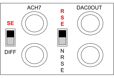
Figure 2: Breakout box switch references. Demonstration of the proper NI 2090A switch positions. Please click here to view a larger version of this figure.

2. Visual stimulation utilizing the VE2020 visual displays and VE2020 LED targets

1. Begin the calibration of the VisualEyes2020 stimulus display(s).
   1. Open the virtual instrument (VI) file named Pix2Deg2020.vi. Select the monitor to be calibrated by utilizing the stretch mode ID input field and the monitor's corresponding display index (Figure 3).
   2. Select a stimulus image (e.g., RedLine.bmp) by typing the stimulus filename into the Line input field.
      NOTE: It is important to note that Pix2Deg2020.vi utilizes .bmp files, not .dds files.
   3. Run Pix2Deg2020.vi, and adjust the stimulus position until it superimposes on a measured physical target.
   4. Once the virtual image aligns with the physically measured target, record the on-screen pixel value for the given degree value. Record a minimum of three calibration points with varying stimulated degree demands and their corresponding pixel values.
   5. Ensure that after recording each calibration point, VE2020 produces an output file named Cals.xls. Utilizing the calibration points in Cal.xls, apply a best-fit linear regression to map the experimentally required eye movement stimulus demands, in degrees of rotation, into pixels. An example five-point degree to recorded pixel calibration is shown in Figure 4.
2. Repeat this procedure for different stimulus images (i.e., the background or second visual stimulus, as necessary) and each stimulus monitor that is expected to be utilized.

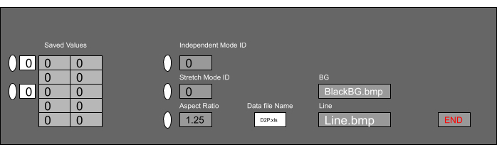
Figure 3: Stimulated degrees to monitor pixels. Depiction of the operator view for calibrating the VE2020. From left to right, a table of values for the recorded pixels corresponding to a known degree value is provided for a given stimulus monitor selection (stretch mode ID) with a fixed aspect ratio, given file name, background stimulus (BG), and foreground stimulus (Line). Please click here to view a larger version of this figure.

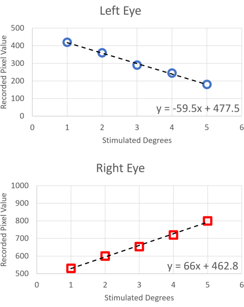
Figure 4: Pixel to degree calibration slopes. Monocular calibration curve for known degree values and measured pixel values. Please click here to view a larger version of this figure.

3. LED calibration

1. Determine the experimental degrees of rotation by utilizing trigonometric identities in the vertical or horizontal planes (Figure 5). Plot the degrees of rotation as a function of the LED number.
2. Linearly regress the LED number as a function of the degrees of rotation. Use the obtained relationship to calculate the initial and final LED numbers, which will be used as visual stimuli during the experiment.

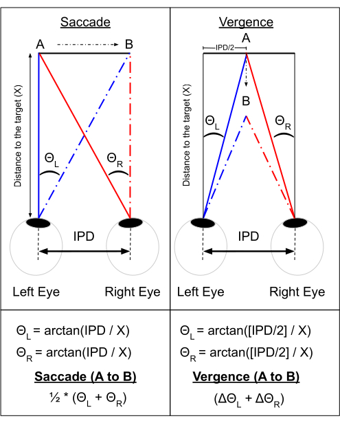
Figure 5: Calculated degrees of rotation. Method of calculating the angular displacement for both saccadic eye movements and vergence movements with a known distance to the target (X) and inter-pupillary distance (IPD). Please click here to view a larger version of this figure.

4. Software programming

1. Define the VisualEyes display input file, and save it to the stimulus library as follows.
   1. To define each stimulus, open a new text (.txt) file prior to the experiment. On the first row of this text file, confirm the presence of four required tab-delimited parameters: stimulus timing (s); X-position (pixels); Y-position (pixels); and rotation (degrees). Additionally, confirm the presence of two optional successive parameters: scaling X (horizontal scaling); and scaling Y (vertical scaling).
   2. Calculate the pixel value for each desired stimulus degree by utilizing the linear regression equation derived from the calibration (see step 2.1.5).
   3. Confirm within the next row of the text file that the length (s) for which the stimulus is presented at its initial position and subsequent final position are present and tab-delimited.
   4. Save the stimulus file in the directory as a VisualEyes input (VEI) file with an informative file name (e.g., stimulus_name_movement_size.vei).
      NOTE: Each stimulus file is positioned monocularly, so a separate file must be generated for the complementary eye to evoke a binocular movement.
2. Repeat these procedures for each desired experimental stimulus, respective movement type, movement magnitude, and eye as appropriate.

5. DC files

1. Create a stimulus library for each stimulus monitor. Name these libraries as dc_1.txt through dc_7.txt. For the settings contained within the dc_1.txt and dc_2.txt files, reference Table 2.
   1. Validate the numerical ID for each stimulus monitor by clicking on Display > Screen Resolution > Identify. Ensure that the device ID is the primary GPU (starting index 0) and that the window mode is 1.
   2. Verify that left defines the left boundary of the screen (in pixels), top defines the top boundary of the screen (in pixels), width is the longitudinal width of the screen (in pixels), and height is the vertical height of the screen (in pixels).
   3. Establish the stimulus number (Stim#), which associates the stimulus file name and location (.dds) and, provided the nostimulus.vei file is stimulus number zero, associates them to a stimulus index number. For the subsequent stimulus_name.vei, list the various stimulus files that are able to be used within the experimental session.
      NOTE: The nostimulus.vei file is beneficial when using ExpTrial as nostimulus.vei does not present a stimulus (blank screen).

Table 2: DC file configuration. The table provides an overview of the DC text file format. Please click here to download this Table.

6. LED input file definition and stimulus library storing

1. Open a new text (.txt) file, and within the file, utilize tab delimitation. End each line within the text file with two tab-delimited zeros.
2. In the first row, define the initial time (s) and LED (position) values. In the second row, define the final time (s) and final LED position values. Save the stimulus_name.vei file in the directory, and repeat these steps for all stimuli.
3. Once completed, save all the stimulus file(s) into the stimulus library, array_config.txt.
4. Ensure that the first row in the array_config.txt file is the communication (COM) port that VisualEyes uses to communicate with the flexible visual stimulator with the default input value COM1; the second row is the baud rate with the default input value as 9,600; the third row is the data bit capacity with the default input value as 8 bits; and the fourth row is the data parity index with the default input value as 0. The succeeding rows in the file contain the stimulus file of the flexible visual stimulator (Figure 6).
5. Check the profile number, as seen in Figure 6; this refers to the corresponding row index of any given stimulus file name, which starts at index zero.

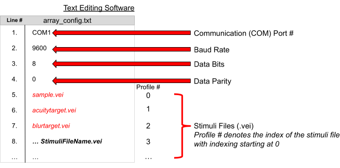
Figure 6: Stimulus library. Utilizing text-editing software, the format shown for identifying the port communications, baud rate, data size, and parity, as well as the library of stimulus files (.vei), provides the VE2020 with the necessary configurations and stimulus file names to run successfully. Please click here to view a larger version of this figure.

7. Script creation for experimental protocols

1. Open a new text (.txt) file to script the experimental protocol commands for VE2020 to read and execute. Check the proper syntax for the experimental protocol commands and documentation. Table 3 provides an overview of the VE2020 syntax conventions.
   NOTE: VE2020 will read these commands sequentially.
2. Save the text file in the directory as a VisualEyes Script (VES), such as script_name.ves. From the previous VisualEyes version manual¹¹, check for a table of software functions that have input and output capabilities. Table 3 demonstrates three newly implemented updated functions.

Table 3: VE2020 function syntax. VE2020 has specific syntax, as demonstrated in the table for calling embedded functions and commenting. Please click here to download this Table.

8. Participant preparation and experiment initiation

1. Acquiring consent and eligibility
   1. Use the following general participant eligibility criteria: aged 18-35 years, 20/25 (or greater) corrected monocular visual acuity, stereo acuity of 500 s (or better) of arc, and 2 weeks (or greater) of utilizing proper refractive correction.
   2. Use the following convergence insufficiency (CI) participant eligibility criteria following established practices¹²: Convergence Insufficiency Symptom Survey (CISS)¹³ score of 21 or greater, failure of Sheard's criterion¹⁴, 6 cm (or greater, at break) near point of convergence (NPC), and 4Δ (or greater) exodeviation (near compared to far).
   3. Use the following control participant eligibility criteria: CISS score less than 21, less than 6Δ difference between near and far phoria, less than 6 cm (at break) NPC, passing of Sheard's criterion, and sufficient minimum amplitude of accommodation as defined by Hofstetter's formula¹⁵.
   4. Use the following general participant ineligibility criteria: constant strabismus, prior strabismus, or refractive surgery, dormant or manifested nystagmus, encephalopathy, diseases that impair accommodative, vergence, or ocular motility, 2Δ (or greater) vertical heterophoria, and inability to perform or comprehend study-related tests. The CI ineligibility criteria further include participants with less than 5 diopters accommodative responses via Donder's push-up method¹⁶.
   5. Once informed consent is acquired, direct the participant to be seated in the haploscope.
   6. Position the participant's forehead and chin against a fixed headrest to minimize head movement, and adjust the participant's chair height so that the participant's neck is in a comfortable position for the entire duration of the experiment.
   7. Adjust the eye movement recording camera(s) to ensure the participant's eyes are captured within the camera's field of view.
2. After being properly seated in the haploscope and eye tracker/autorefractor, ask the participant to visually fixate on a visually presented target. During this setup, ensure the participant's eyes are centered so that visual targets are presented on the midsagittal plane.
   1. Achieve eye centering by having high acuity targets presented binocularly at the visual midline. The participant is aligned at the visual midline when physiological diplopia (double vision) occurs centered around the target of fixation.
3. Then, adjust the eye-tracking gating and eye-tracking signal gains to capture anatomical features such as the limbus (the boundary between the iris and sclera), pupil, and corneal reflection.
4. Validate the capture of the eye movement data by asking the participant to perform repeated vergence and/or saccadic movements.
5. Following the preliminary validation and physical monitor calibrations, open ReadScript.vi. Once ReadScript.vi has opened, select the experimental protocol script by typing in the file name in the top-left corner. Run the protocol via ReadScript.vi by pressing the white arrow in the top-left corner to execute Acquire.vi.
6. Provide the participant with a handheld trigger button, and explain that when the trigger is pressed, the data collection will commence. A file will automatically appear on the control monitor screen, Acquire.vi, which plots a preview of the recorded eye movement data. When the experimental protocol is complete, ReadScript.vi automatically stops, and data output files are automatically generated and stored.

9. VNEL eye movement analysis program (VEMAP)

1. Data preprocessing
   1. Begin the analysis by selecting the Preprocess Data button. A file explorer window will appear. Select one or many recorded data files from VE2020 for preprocessing.
   2. Filter the data with a 20-order Butterworth filter: 40 Hz for vergence eye movements and 120 Hz or 250Hz for saccadic eye movements. The completed preprocessed data files will be stored within the VEMAP Preprocessed folder as .mat files.
      NOTE: The filtering frequency for VEMAP can be adjusted to the user's preferred cut-off frequency, dependent on the application.
2. Calibration
   1. Utilizing the three stimulated monocular calibration movements respectively for the left and right eye positions evoked from the VE2020 script, create a linear regression of the eye movement stimuli in degrees as a function of the recorded voltage values. As shown in the lower plots of Figure 7, use the respective Pearson correlation coefficients and regression formulas for the quantitative assessment of the fitment.
   2. Utilize the slope of each regression as the respective monocular calibration gain to convert the recorded (raw) voltages to degrees (calibrated).
   3. Identify from the experimental calibrations an appropriate gain value for the left and right eye movement responses. Consistently apply the calibration gain to each recorded eye movement stimulus section. Following the calibration of all the movement subsections, a confirmation window will appear.
      NOTE: Monocular eye movement calibrations are chosen due to the potential inability of patients with convergence insufficiency, the primary ocular motor dysfunction investigated by our laboratory, to perceive a binocular calibration as a single percept. If the recorded calibration signals are saturated or not linearly correlated (due to not attending to the stimulus, blinking, saccadic movements, eye tearing, or closure of the eyes), then apply standardized calibration gains for the left and right eye movement responses. This should be done sparingly, and these calibration gain values should be derived from large group-level averages of previous participants for the left and right eye movement response gains, respectively.
3. Classification
   1. Following the calibration, inspect each eye movement response manually, and categorize using a variety of classification labels, such as blink at transient, symmetrical, asymmetrical, loss of fusion, no movement (no response), and saturated eye movement.
   2. Check Figure 8 for reference. The upper (positional data) plot is the response from a 4° symmetrical vergence step stimulus. The combined convergence movement is shown in green, the right eye movement is shown in red. and the left eye movement is shown in blue. The version trace is shown in black. The lower plot shows the first-derivative velocity of the eye movement position response, with the same color pattern as described above.
4. Data analysis
   1. Perform the final step in the VEMAP processing dataflow of data analysis, which is accessible within the VEMAP user interface (UI) as a button and is previewed in Figure 9. Plot the eye movements within a particular stimulus type and classification label together as an ensemble plot, as shown on the right side of Figure 9.
   2. Selectively analyze the subsets of eye movements via their classification labels or holistically without any applied classification filters via the Choose Classes button.
   3. Check that the primary eye movement metrics correspond to each recorded eye movement, such as the latency, peak velocity, response amplitude, and final amplitude.
   4. Inspect each eye movement response to ensure that each recorded metric is valid. If a metric does not appear appropriate, remeasure the recorded metrics accordingly until appropriate values accurately reflect each movement. In addition, omit eye movements or reclassify their provided classification labels via the Reclassify button if the recorded metrics cannot adequately describe the recorded eye movement.

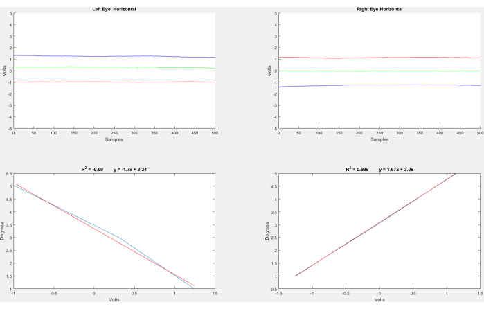
Figure 7: Monocular calibration and correlation slopes. An example of the calibration of eye movement data from voltage values to degrees of rotation. Please click here to view a larger version of this figure.

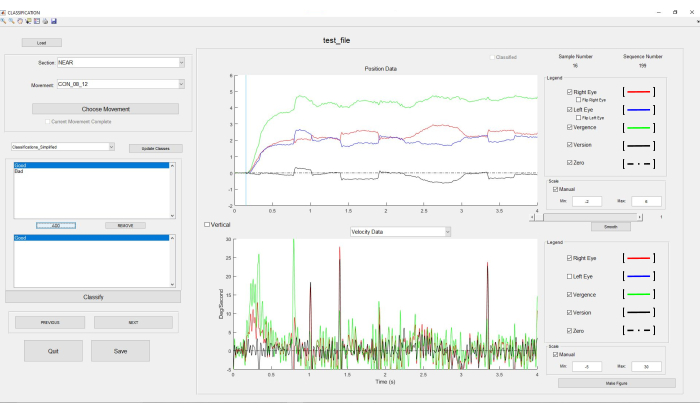
Figure 8: Eye movement software classification. Classification of the stimulated eye movement responses. Please click here to view a larger version of this figure.

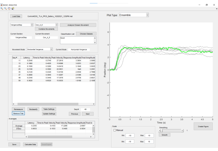
Figure 9: Eye movement response software analysis. An example of plotted convergence responses stimulated by a 4° symmetrical step change (right), with individual eye movement response metrics presented tabularly (left) and group-level statistics displayed tabularly below the response metrics. Please click here to view a larger version of this figure.

10. Accommodative Movement Analysis Program (AMAP)

1. Data configuration
   1. Utilizing the external storage device that contains the autorefractor data, export the data to a device with the AMAP installed. The AMAP is available as a standalone executable as well as a local application via the MATLAB application installation.
2. Start the AMAP application. From the AMAP, select either File Preprocessor or Batch Preprocessor. The file preprocessor processes an individual data folder, while the batch preprocessor processes a selected data folder directory.
3. Check the AMAP's progress bar and notifications, as the system provides these when the selected data have been preprocessed. Folder directories are generated from the AMAP's preprocessing for data processing transparency and accessibility via the computer's local drive under AMAP_Output.
4. If an AMAP feature is selected without prior data processing, check for a file explorer window that appears for the user to select a data directory.
5. Perform the AMAP data analysis as described below.
   1. Following preprocessing, select a data file to analyze via the Load Data button. This will load any available files into the current file directory defaulted to a generated AMAP_Output folder. The selected data filename will be shown in the current file field.
   2. Under the eye selector, check the default selection, which presents binocularly averaged data for the recorded accommodative refraction.
   3. Switch the data type between accommodative refraction and oculomotor vergence (gaze) via the Type Selector. Check further graphical customizations available to present the data metrics and first-order and second-order characterizations. Check Figure 10 for the combinations of graphical options that can be selected for the operator to visualize.
   4. Check the default metrics for the AMAP, which are as follows: peak velocity (degrees/s); response amplitude (degrees); final amplitude (degrees); response starting index (s); peak velocity index (s); response ending index (s); gaze (vergence) velocity (degrees/s); gaze response amplitude (degrees); gaze final amplitude (degrees); gaze response starting index (s); gaze velocity index (s); gaze response ending index (s); and classification (binary 0 - bad, 1 - good).
   5. Perform modifications to the response starting index, response ending index, and peak velocity index through the metric modification spinners (Figure 10).
   6. Following the analysis of all the recorded movements displayed, save the analyzed metrics for each data file in the movement ID field or via the leftward and rightward navigation arrows.
   7. Select the Save button to export the analyzed data to an accessible spreadsheet. Unanalyzed movements have a default classification of not-a-number (NaN) and are not saved or exported.
   8. Perform manual classification (good/bad) for each movement to ensure complete analysis by any operator.

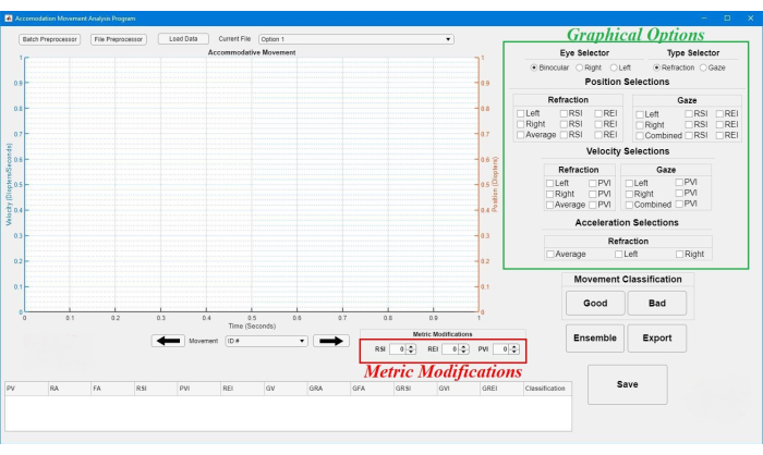
Figure 10: AMAP software frontend. The figure displays the main user interface for the AMAP with highlighted sections for the graphical presentation (graphical options) of data and data analysis (metric modifications). Please click here to view a larger version of this figure.

Results

Group-level ensemble plots of stimulated eye movements evoked by VE2020 are depicted in Figure 11 with the corresponding first-order velocity characteristics.

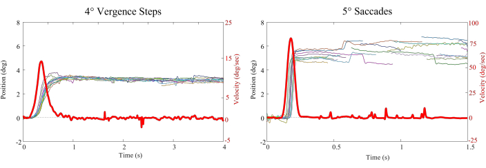
Figure 11

Discussion

Applications of the method in research
Innovations from the initial VisualEyes2020 (VE2020) software include the expansibility of the VE2020 to project onto multiple monitors with one or several visual stimuli, which allows the investigation of scientific questions ranging from the quantification of the Maddox components of vergence¹⁸ to the influence of distracting targets on instructed targets¹⁹. The expansion of the haploscope system to VE2020 alon...

Materials

List of materials used in this article

Name	Company	Catalog Number	Comments
Analog Terminal Breakout Box	National Instruments	2090A
Convex-Sphere Trial Lens Set	Reichert	Portable Precision Lenses	Utilized for autorefractor calibration
Graphics Cards	-	-	Minimum performance requirement of GTX980 in SLI configuration
ISCAN Eye Tracker	ISCAN	ETL200
MATLAB	MathWorks	v2022a	AMAP software rquirement
MATLAB	MathWorks	v2015a	VEMAP software requirement
Microsoft Windows 10	Microsoft	Windows 10	Required OS for VE2020
Plusoptix PowerRef3 Autorefractor	Plusoptix	PowerRef3
Stimuli Monitors (Quantity: 4+)	Dell	Resolution 1920x1080	Note all monitors should be the same model and brand to avoid resolution differences as well as physical configurations

References

- Alvarez, T. L., et al. Disparity vergence differences between typically occurring and concussion-related convergence insufficiency pediatric patients. Vision Research. 185, 58-67 (2021).
- Alvarez, T. L., et al. Underlying neurological mechanisms associated with symptomatic convergence insufficiency. Scientific Reports. 11, 6545(2021).
- Scheiman, M., Kulp, M. T., Cotter, S. A., Lawrenson, J. G., Wang, L., Li, T. Interventions for convergence insufficiency: A network meta-analysis. The Cochrane Database of Systematic Reviews. 12 (12), (2020).
- Semmlow, J. L., Chen, Y. F., Granger-Donnetti, B., Alvarez, T. L. Correction of saccade-induced midline errors in responses to pure disparity vergence stimuli. Journal of Eye Movement Research. 2 (5), (2009).
- Scheiman, M., Wick, B. Clinical Management of Binocular Vision., 5th Edition. , Lippincott Williams & Wilkins. Philadelphia, USA. (2019).
- Kim, E. H., Vicci, V. R., Granger-Donetti, B., Alvarez, T. L. Short-term adaptations of the dynamic disparity vergence and phoria systems. Experimental Brain Research. 212 (2), 267-278 (2011).
- Labhishetty, V., Bobier, W. R., Lakshminarayanan, V. Is 25Hz enough to accurately measure a dynamic change in the ocular accommodation. Journal of Optometry. 12 (1), 22-29 (2019).
- Juhola, M., et al. Detection of saccadic eye movements using a non-recursive adaptive digital filter. Computer Methods and Programs in Biomedicine. 21 (2), 81-88 (1985).
- Mack, D. J., Belfanti, S., Schwarz, U. The effect of sampling rate and lowpass filters on saccades - A modeling approach. Behavior Research Methods. 49 (6), 2146-2162 (2017).
- Ghahghaei, S., Reed, O., Candy, T. R., Chandna, A. Calibration of the PlusOptix PowerRef 3 with change in viewing distance, adult age and refractive error. Ophthalmic & Physiological Optics. 39 (4), 253-259 (2019).
- Guo, Y., Kim, E. L., Alvarez, T. L. VisualEyes: A modular software system for oculomotor experimentation. Journal of Visualized Experiments. (49), e2530(2011).
- Convergence Insufficiency Treatment Trial Study Group. Randomized clinical trial of treatments for symptomatic convergence insufficiency in children. Archives of Ophthalmology. 126 (10), 1336-1349 (2008).
- Borsting, E., et al. Association of symptoms and convergence and accommodative insufficiency in school-age children. Optometry. 74 (1), 25-34 (2003).
- Sheard, C. Zones of ocular comfort. American Journal of Optometry. 7 (1), 9-25 (1930).
- Hofstetter, H. W. A longitudinal study of amplitude changes in presbyopia. American Journal of Optometry and Archives of American Academy of Optometry. 42, 3-8 (1965).
- Donders, F. C. On the Anomalies of Accommodation and Refraction of the Eye. , Milford House Inc. Boston, MA. translated by Moore, W. D (1972).
- Sravani, N. G., Nilagiri, V. K., Bharadwaj, S. R. Photorefraction estimates of refractive power varies with the ethnic origin of human eyes. Scientific Reports. 5, 7976(2015).
- Maddox, E. E. The Clinical Use of Prisms and the Decentering of Lenses. , John Wright and Co. London, UK. (1893).
- Yaramothu, C., Santos, E. M., Alvarez, T. L. Effects of visual distractors on vergence eye movements. Journal of Vision. 18 (6), 2(2018).
- Borsting, E., Rouse, M. W., De Land, P. N. Prospective comparison of convergence insufficiency and normal binocular children on CIRS symptom surveys. Convergence Insufficiency and Reading Study (CIRS) group. Optometry and Vision Science. 76 (4), 221-228 (1999).
- Maxwell, J., Tong, J., Schor, C. The first and second order dynamics of accommodative convergence and disparity convergence. Vision Research. 50 (17), 1728-1739 (2010).
- Alvarez, T. L., et al. The Convergence Insufficiency Neuro-mechanism in Adult Population Study (CINAPS) randomized clinical trial: Design, methods, and clinical data. Ophthalmic Epidemiology. 27 (1), 52-72 (2020).
- Leigh, R. J., Zee, D. S. The Neurology of Eye Movements. , Oxford Academic Press. Oxford, UK. (2015).
- Alvarez, T. L., et al. Clinical and functional imaging changes induced from vision therapy in patients with convergence insufficiency. Annual International Conference of the IEEE Engineering in Medicine and Biology Society. 2019, 104-109 (2019).
- Scheiman, M. M., Talasan, H., Mitchell, G. L., Alvarez, T. L. Objective assessment of vergence after treatment of concussion-related CI: A pilot study. Optometry and Vision Science. 94 (1), 74-88 (2017).
- Yaramothu, C., Greenspan, L. D., Scheiman, M., Alvarez, T. L. Vergence endurance test: A pilot study for a concussion biomarker. Journal of Neurotrauma. 36 (14), 2200-2212 (2019).
Access restricted. Please log in or start a trial to view this content.
Reprints and Permissions