JoVE Science Education
Biomedical Engineering
A subscription to JoVE is required to view this content.  Sign in or start your free trial.
JoVE Science Education Biomedical Engineering
Quantitative Strain Mapping of an Abdominal Aortic Aneurysm
  • 00:07Overview
  • 01:14Principles of Strain Mapping
  • 03:404D Ultrasound Set-up
  • 04:58Ultrasound Image Acquisition
  • 05:45Image Analysis
  • 07:30Results
  • 08:41Applications
  • 10:02Summary

Mapeamento Quantitativo de Tensão de um Aneurisma da Aorta Abdominal

English

Share

Overview

Fonte: Hannah L. Cebull1, Arvin H. Soepriatna1, John J. Boyle2 e Craig J. Goergen1

1 Weldon School of Biomedical Engineering, Purdue University, West Lafayette, Indiana

2 Engenharia Mecânica & Ciência dos Materiais, Universidade de Washington em St. Louis, St Louis, Missouri

O comportamento mecânico dos tecidos moles, como vasos sanguíneos, pele, tendões e outros órgãos, são fortemente influenciados por sua composição de elastina e colágeno, que proporcionam elasticidade e força. A orientação de fibras dessas proteínas depende do tipo de tecido mole e pode variar de uma única direção preferencial a redes intrincadas de malha, que podem se tornar alteradas em tecido doente. Portanto, os tecidos moles muitas vezes se comportam anisotropicamente no nível celular e órgão, criando uma necessidade de caracterização tridimensional. Desenvolver um método para estimar de forma confiável os campos de cepas dentro de tecidos ou estruturas biológicas complexas é importante para caracterizar e entender a doença mecanicamente. A cepa representa como o tecido mole se deforma relativamente ao longo do tempo, e pode ser descrito matematicamente através de várias estimativas.

A aquisição de dados de imagem ao longo do tempo permite que a deformação e a tensão sejam estimadas. No entanto, todas as modalidades de imagem médica contêm alguma quantidade de ruído, o que aumenta a dificuldade de estimar com precisão a tensão in vivo. A técnica aqui descrita supera esses problemas com sucesso usando um método de estimativa de deformação direta (DDE) para calcular campos de cepa 3D espacialmente variados a partir de dados de imagem volumosas.

Os métodos atuais de estimativa de tensão incluem correlação de imagem digital (DIC) e correlação de volume digital. Infelizmente, o DIC só pode estimar com precisão a tensão de um plano 2D, limitando severamente a aplicação deste método. Embora úteis, métodos 2D como DIC têm dificuldade em quantificar a cepa em regiões que sofrem deformação 3D. Isso ocorre porque o movimento fora do avião cria erros de deformação. A correlação de volume digital é um método mais aplicável que divide os dados de volume inicial em regiões e encontra a região mais semelhante do volume deformado, reduzindo assim o erro fora do plano. No entanto, este método se mostra sensível ao ruído e requer suposições sobre as propriedades mecânicas do material.

A técnica aqui demonstrada elimina essas questões utilizando um método DDE, tornando-o muito útil na análise de dados de imagem médica. Além disso, é robusto para tensão alta ou localizada. Aqui descrevemos a aquisição de dados de ultrassom 4D fechados, volumétricos, sua conversão em um formato analisável e o uso de um código Matlab personalizado para estimar a deformação 3D e as cepas verdes-lagrange correspondentes, um parâmetro que melhor descreve grandes deformações. O tensor de cepa Green-Lagrange é implementado em muitos métodos de estimativa de cepas 3D porque permite que f seja calculado a partir de um Ajuste De Menor Quadrado (LSF) dos deslocamentos. A equação abaixo representa o tensor de cepa Green-Lagrange, E, onde F e I representam o gradiente de deformação e tensor de identidade de segunda ordem, respectivamente.
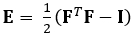
Equation 1 (1)

Principles

Procedure

1. Configuração de ultrassom 4D Ao usar o software de imagem, use um laptop capaz de executar software matemático de computação para automatizar o processo de aquisição 4D. Conecte o laptop com este código personalizado ao sistema de ultrassom através da porta USB. Observe que o software de imagem tem um recurso de ultrassom 4D integrado ao software. Depois de ligar o sistema de ultrassom, configure a unidade de monitoramento fisiológico e, ao mesmo tempo, garanta que os botões de frequênc…

Results

Using the procedure described above, 4D ultrasound of an angiotensin II-induced suprarenal dissecting abdominal aortic aneurysm (AAA) of a mouse was acquired. Multiple short-axis EKV video loops were acquired along the aorta and combined to create 4D data, as shown in Figure 1. This data was then converted into a MAT file using a custom code, which was then analyzed in a 3D strain calculation code using a warping function. After optimizing the parameters of the code for a specific data set, a representative, long-axis view with corresponding strain values was produced as well as a 3D slice visualization plot with an overlaid strain color map (Figure 2). This DDE technique and strain data highlight the heterogeneous spatial variations in strain, particularly when a thrombus is present. These results can then be correlated with vessel structure to determine the relationship between in vivo deformation and aneurysm composition.

Equation 3
Figure 1: ECG-gated kilohertz visualization (EKV) loops of the aorta are acquired from manually inputted starting and ending locations, following a step size of 0.2 mm.

Figure 1
Figure 2: 4D high frequency ultrasound data of a murine dissecting abdominal aortic aneurysm represented at systole (A) with principal strain fields estimated and overlaid (B) (Scalebar = 5 mm). Long- and short-axis views representing both aneurysmal and healthy regions corresponding principal strain over one cardiac cycle (systole: t= 0.4) (C, D). These data show relatively high strain levels in healthy regions and reduced strain values within the dissecting aneurysm.

Applications and Summary

Localized in vivo mechanical characterization is an important part of understanding the growth and remodeling of biological tissues. Compared to existing approaches, the strain quantification procedure described here uses an improved method of accurately calculating 3D strain through optimally warping the undeformed image before cross-correlation. This method does not use any material assumptions in determining strains within tissue volumes. Unfortunately, the strain estimation is reliable only down to a kernel size of 15x15x15 voxels when using ultrasound data, suggesting that this DDE approach may not detect subtle features within a strain field. Despite this limitation, it remains an important tool for investigating mechanical responses, diagnosing pathology, and improving disease models.

Many areas of research beyond aortic aneurysms can benefit from this strain measurement tool. Cardiac strain can also be easily quantified using this method. Because the myocardium undergoes 3D deformation during the cardiac cycle, quantifying strain in three dimensions is integral to reliably characterizing the dynamics of this tissue. Reliable strain data is especially important when tracking disease progression in animal models.

3D strain analysis can also be applied to intestinal ultrasound imaging. Mechanical characterization of intestinal tissue is most commonly conducted in vitro. However, this is not always a true representation of the actual behavior of the intestines in vivo because of effects from surrounding structures. As an example of clinically translating this approach, calculating the strain from images of intestinal fibrosis due to abnormal luminal pressure could provide early detection of problematic areas that require surgical intervention.

Beyond the larger scale applications, this method can also be applied to the cellular level by using higher resolution imaging techniques, such as confocal microscopy. Characterizing the extracellular matrix is important for understanding how cells communicate. Much research has been conducted on the biochemical characterization, but understanding how communication can be conducted through mechanical responses requires an understanding of deformation and strain. Bulk strain is not beneficial because there is no way to determine the origin of the deformation change. Applying a high-resolution DDE approach could directly reveal how the extracellular matrix responds to mechanical changes.

ACKNOWLEDGEMENTS

We would like to acknowledge John Boyle, Guy Genin, and Stavros Thomopoulos for the contribution of the DDE custom Matlab code capable of directly estimating Lagrange-Green strain.

Transcript

Three-dimensional strain imaging is used to estimate deformation of soft tissues over time and understand disease. The mechanical behavior of soft tissues, such as skin, blood vessels, tendons, and other organs, is strongly influenced by their extracellular composition, which can become altered from aging and disease. Within complex biological tissues, it is important to characterize these changes, which can significantly affect the mechanical and functional properties of an organ.

Quantitative strain mapping uses volumetric image data and a direct deformation estimation method to calculate the spatially varying three-dimensional strain fields. This video will illustrate the principles of strain mapping, demonstrate how quantitative strain mapping is used to estimate strain fields within complex biological tissues, and discuss other applications.

Biological tissues are strongly influenced by the composition and orientation of elastin and collagen. The protein elastin is a highly elastic component of tissues that continually stretch and contract, such as blood vessels and the lungs. Collagen is the most abundant protein in the body, and is assembled from individual triple-helical polymers that are bundled into larger fibers that provide structural integrity to tissues ranging from skin to bones.

The orientation of these proteins ranges from aligned fibers to fibrous mesh networks, which affects the mechanical properties of the tissue. Strain is a measure of the relative deformation of soft tissues over time, and can be used to visualize injury and disease. It is described and mapped using mathematical estimations.

To map strain in complex organs, such as the heart, four-dimensional ultrasound data, which provides high resolution, spatial, and temporal information, can be used. Then the direct deformation estimation method, or DDE, is applied to the data. A code is used to estimate the 3D deformation and corresponding Green-Lagrange strains using the following equation.

The Green-Lagrange strain tensor depends on the deformation gradient tensor and the second order identity tensor. Deformation gradient tensors are traditionally estimated from displacement fields. In the DDE method, a warping function is optimized to be directly analogous to the deformation tensor. The warping function depends on both spatial position and the warping parameter. The calculation of deformation is directly incorporated into the warping function. The first nine elements represent the deformation gradient tensor.

This method is used to estimate both large and localized deformations in soft tissues. Now that we understand the principles of strain mapping, let’s now see how strain mapping is performed to detect aortic aneurysms in mice.

To begin setup, open the Vivo 2100 software and connect the laptop to the ultrasound system. Make sure the physiological monitoring unit is on to measure heart rate and temperature. Then initialize the 3D motor stage.

Install the ultrasound transducer and ensure that all proper connections are made. Next, anesthetize the animal that will be imaged using 3% isoflurane in a knock-down chamber. Once the mouse is anesthetized, move it to the heated stage and secure a nose cone to deliver 1-2% isoflurane. Apply ophthalmic ointment to the eyes and secure the paws to the stage electrodes to monitor the animal’s respiration and heart rate. Then insert a rectal temperature probe. Apply depilatory cream to remove hair from the area of interest, and then apply a generous amount of warm ultrasound gel to the depilated area.

To start the image acquisition, first, open the imaging window and select B mode. Then lower the transducer onto the animal and use the x and y-axis knobs on the stage to locate the area of interest. Monitor the respiratory rate to make sure it does not decrease substantially. Position the transducer in the middle of the region of interest. Then approximate the distance required to cover the entire region of interest.

Enter these dimensions in the MATLAB code and choose a step size of 0.08 millimeters. Make sure the animal’s heart and respiratory rates are stable, then run the MATLAB code.

After image acquisition, export the data as raw XML files and convert them into MAT files. Make sure to input the number of frames, step size, and output resolution. Then re-sample the matrix in through-plane.

Import the new MAT file into the 3D strain analysis code. It may be necessary to rescale the file to reduce the computation time. Then, input the region to be analyzed. Approximate the number of pixels in a two-dimensional slice of the tracked feature and select the mesh template either as a simple box or manually chosen polygons. Choose the optimal pixel number for the mesh size. Compute the Jacobians and the gradients. Repeat for each region. Then apply the warping function.

Next, using Cartesian deformations calculated from DDE, determine the eigenvalues and eigenvectors of the deformation. Then, select the slices that you want to plot strain values for by scrolling through the long axis, sort axis, and coronal axis views.

Press Select Manifold for Analysis. Then use the cursor to place markers along the aortic wall, including the thrombus, aneurysm, and healthy parts of the aorta. Repeat for all views. Finally, use color mapping to plot the results of the strain field over the region of interest.

Let us have a close look at the example of an angiotensin II-induced suprarenal dissecting abdominal aortic aneurysm acquired from a mouse. First, multiple short axis ECG-gated kilohertz visualization loops are obtained at a given step size along the aorta and combined to create 4D data.

After performing 3D strain calculation using an optimized warping function, the 3D slice visualization plot of the infrarenal aorta is obtained. The color map of principal green strain is overlaid to highlight regions of heterogeneous aortic wall strain. In addition, long axis and short axis views reveal heterogeneous spatial variations in strain, particularly when a thrombus is present.

Corresponding strain plots show higher strain values in healthy regions of the aorta in the long axis, while the aneurysmal region shows decreased strain in the short axis.

Accurate quantitative strain visualization using direct deformation estimation is a useful tool used in various biomedical applications.

For instance, cardiac strain can be quantified. During the cardiac cycle, the myocardium undergoes 3D deformation. Quantifying strain in three dimensions is integral to reliably characterizing the dynamics of this tissue over time. This is useful in tracking disease progression in animal models.

Another application is in the characterization of intestinal tissue. In vivo imaging of the intestines is challenging because of the effects from surrounding structures. However, calculating strain from images of intestinal fibrosis could be particularly useful to provide early detection of problematic areas that require surgical intervention.

At a much smaller scale, this DDE method is also applied to the cellular level by using higher resolution imaging techniques such as confocal microscopy. It serves, for example, in the characterization of extracellular matrix to understand how cells communicate under mechanical changes.

You’ve just watched JoVE’s introduction to quantitative strain visualization. You should now understand how to measure three-dimensional strain in biological tissues and how that is used in early disease detection. Thanks for watching!

Tags

Cite This
JoVE Science Education Database. JoVE Science Education. Quantitative Strain Mapping of an Abdominal Aortic Aneurysm. JoVE, Cambridge, MA, (2023).