Quantifying Mixing using Magnetic Resonance Imaging

Summary

Magnetic resonance imaging (MRI) provides a powerful tool to evaluate the effectiveness of process equipment during operation. We discuss the use of MRI to visualize mixing in a static mixer. The application is relevant to personal care products, but can be applied to a broad range of food, chemical, biomass and biological fluids.

Abstract

Mixing is a unit operation that combines two or more components into a homogeneous mixture. This work involves mixing two viscous liquid streams using an in-line static mixer. The mixer is a split-and-recombine design that employs shear and extensional flow to increase the interfacial contact between the components. A prototype split-and-recombine (SAR) mixer was constructed by aligning a series of thin laser-cut Poly (methyl methacrylate) (PMMA) plates held in place in a PVC pipe. Mixing in this device is illustrated in the photograph in Fig. 1. Red dye was added to a portion of the test fluid and used as the minor component being mixed into the major (undyed) component. At the inlet of the mixer, the injected layer of tracer fluid is split into two layers as it flows through the mixing section. On each subsequent mixing section, the number of horizontal layers is duplicated. Ultimately, the single stream of dye is uniformly dispersed throughout the cross section of the device.

Using a non-Newtonian test fluid of 0.2% Carbopol and a doped tracer fluid of similar composition, mixing in the unit is visualized using magnetic resonance imaging (MRI). MRI is a very powerful experimental probe of molecular chemical and physical environment as well as sample structure on the length scales from microns to centimeters. This sensitivity has resulted in broad application of these techniques to characterize physical, chemical and/or biological properties of materials ranging from humans to foods to porous media ^{1, 2}. The equipment and conditions used here are suitable for imaging liquids containing substantial amounts of NMR mobile ¹H such as ordinary water and organic liquids including oils. Traditionally MRI has utilized super conducting magnets which are not suitable for industrial environments and not portable within a laboratory (Fig. 2). Recent advances in magnet technology have permitted the construction of large volume industrially compatible magnets suitable for imaging process flows. Here, MRI provides spatially resolved component concentrations at different axial locations during the mixing process. This work documents real-time mixing of highly viscous fluids via distributive mixing with an application to personal care products.

Protocol

1. Mixer design

1. Use a CAD program to design the mixing sections of the static mixer.

The SAR mixer is composed of a number of different plate geometries; these geometries are shown in Fig. 3. Each laser-cut Poly (methyl methacrylate) (PMMA) plate is 1.59 mm thick and has a rectangular key at the bottom so that it can be aligned in a PVC pipe with an acrylic rod. The geometry is similar to those described in [3, 4], except that the walls in the expansions and contractions are formed by a series of discrete “staircase” steps due to the alignment of discrete plates rather than smooth diagonal surfaces. Although the material of construction here is PMMA and PVC, opaque non-metallic mixers can be constructed as well.

2. Align the individual plates to develop the repeating units of the mixer. Position the plates tightly within a 1½ inch Schedule 40 clear PVC pipe.
3. Fig. 4 illustrates the static mixer viewed from the side. Notice that two fluids enter at the left side of the figure. The minor component, shown as the dark region, enters through the nozzle (Plate S, Fig. 3) and forms a stream of the minor component in the (colorless) major component. The repeating unit starts after Plate S at the first Plate C and extends downstream through Plate 48, which is also a Plate C. In each repeating unit, the two fluids flow into 8 plates of open channel (Plate C). The fluid is then physically separated into two vertical channels by eight plates of Plate I, followed by the actual mixing section. The mixing section is a total of 16 plates, from upstream to downstream: Plates I, A, B, D, E, F, G, J, J, K, L, M, N, O, P, and H. The fluid leaves the mixing section and flows into 8 plates of Plate H, in which fluid is physically split into two horizontal channels. The “H” section is followed by 8 plates of open channel (Plate C). This pattern of 48 plates is repeated 6 times in the mixer. Two repeating units are illustrated in Fig. 4 as Plates 1-96.

2. Flow system with MR imaging system and a mixer

1. Assemble a flow system to pump Carbopol solution through the in-line split-and-recombine static mixer. Be able to control and record the mass flow rate of the test fluids. In addition, incorporate a pressure transducer upstream of the mixer to monitor pressure.
2. Position the mixer in the magnet (Fig. 5). The magnet is part of a 1 Tesla permanent-magnet-based imaging spectrometer (Aspect Imaging, Industrial Area Hevel Modi'in, Shoham, Israel), with 0.3 T/m peak gradient strength The dimensions of the magnet enclosure are 700 x 700 x 600 mm.
3. Dope part of the Carbopol solution with manganese chloride (MnCl₂). This will be the minor component. The major component is undoped Carbopol solution. Fig. 6 illustrates a schematic of flow system.

3. Characterization of the test fluid

1. Prepare a 0.2 % w/w Carbopol (The Lubrizol Corporation) solution by slowly sifting a weighed amount of polymer into deionized water in a stirred tank. This polymer family of products is based on crosslinked acrylic acid chemistry and is widely used in personal care and household products as rheological modifiers. Neutralize the carbopol solution with a 50% NaOH solution to pH 7; the neutralization allows the solution to achieve its maximum viscosity as the polymer swells in water to form a gel. Prepare a second carbopol solution containing the MR contrast agent MnCl₂ to a final concentration of 0.040 mM; this solution is referred to as the doped tracer fluid.
2. Characterize the flow behavior, or rheology, of the carbopol solutions with a TA Instruments AR-G2 rheometer (New Castle, DE) with a standard Couette geometry (14 mm diam. x 42 mm height) at a fluid temperature of 25 °C. For shear viscosity, use a steady state shear stress sweep from 0.1 500 Pa in logarithmic mode with 10 points/decade and 5% tolerance. Methods are described in [5].

In this work, the rheological properties of the two solutions were indistinguishable and are illustrated in Fig. 7, data were fit to a power law model and show shear thinning behavior.

Characterize the viscoelastic properties of the 0.2% w/w carbopol solution with small amplitude oscillatory testing. Perform the dynamic testing at a fixed stress of 1 Pa, which corresponds to the linear viscoelastic region. Measure strain over a frequency sweep from 628 - 0.63 rad/s (100-0.10 Hz) in logarithmic mode with 10 points/decade.

The storage and loss moduli, G’ and G” respectively, are shown in Fig. 8. The curves are characteristic of a gel system with G’>G” and G’ fairly constant [5]. Values of tan(δ) = G”/G’ increase from 0.05 at lower frequencies to 0.3 − 0.5 at higher frequency. The corresponding phase lag (δ) followed the same trend, with the limits being δ=0 for Hookean solids and δ=π/2 for Newtonian fluids.

3. Evaluate the relative contribution of viscous forces to inertial forces during flow using the Reynolds number. Since the cross section of each plate varies, the average flow rate through the plate and the Reynolds number is calculated and given in Table 1.

These Reynolds number values are much less than 1.0 and characterize flows in which viscous forces dominate the inertial forces. In other words, the mixing is by laminar stretching and shearing rather than turbulence.

4. MR data acquisition

1. Select an appropriate radio frequency coil.

This work uses a solenoid with four turns, encasing a cylindrical volume 60 mm in diameter and 60 mm long. This coil closely fits the PVC pipe and achieved a good signal-to-noise ratio of the signal.

2. Run a multi-slice gradient echo sequence and acquire MR images.

This pulse sequence was chosen since the signal intensity is sensitive to material spin-lattice relaxation time. The relative signal intensity between two materials with different relaxation times is calculated from an equation. The signal intensity differences, total acquisition time for the image relative to the influence of molecular diffusion during the image acquisition all need to be considered in selecting the appropriate experimental parameters. Additionally, the concentration of the contrast agent (MnCl₂) is chosen such that the signal intensity changes resulting from contrast agent concentration are linear. The addition of MnCl₂ decreases the spin-lattice relaxation time (T₁) of the test fluid from 2.998 s (undoped) to 0.515 s (doped). The doped Carbopol solution appears brighter than the undoped Carbopol solution in the images since the intensity is highly weighted by the spin lattice relaxation time. The pulse sequence parameters are an echo time (TE) of 2 ms and a repetition time (TR) of 30 ms; the field of view (FOV) is 64 mm per 128 encodings which yields an in-plane spatial resolution of 0.5 mm/voxel. With this multi-slice sequence, we acquire 32 cross sectional slices of thickness 1.4 mm per imaging slice.

5. Imaging the fluid

1. Pump both the major and minor components through the mixer until steady flow is achieved. The relative flow rate of the major and minor components is 10:1. Simultaneously stop the pumps and image the fluid in the mixer. The MR sequence does not include flow compensation; to avoid motion artifacts, the imaging is performed on quiescent liquid. Imaging time is on the order of 1-4 minutes.
2. Reposition the mixer several times to image cylindrical volumes at different axial locations.

In this study, several cylindrical volumes of the mixer are imaged and can be located in Fig. 9. The volume is chosen by sliding the mixer tube axially through the magnet, until the desired volume is in the sweet spot defined by the center of the NMR coil in the center of the magnet.

3. Analyze the MR data with image analysis procedures to document the spatial distribution of component concentrations. The relationship between normalized signal intensity (x) and the fraction of doped fluid (y) in this study is y=1.419x-0.482 (R²=0.99). This relationship is relevant to analyze the mixing process.To illustrate the power of flow visualization using MRI, the following results are selected images at different axial locations.

6. Representative Results

Figure 10 illustrates images at the slit nozzle (injector) to show the cross sections as doped and undoped enter the first repeating unit. These images also clearly show the difference in signal intensity between 100% doped fluid and undoped fluid.

The SAR mixer effectively and uniformly splits flow as illustrated in the images of the H Platesdownstream from the 1^st, 2^nd, and ^3rd mixing sections (Fig. 11, first row). The number of doped fluid “stripes” double through each mixing section. The second row of Fig. 11 illustrates the image analysis procedure that thresholds the images to “1”s (stripes) and “0”s (everything else). These processed images clearly illustrate the increase of interfacial area between the doped and undoped fluids as the fluid splits and recombines.

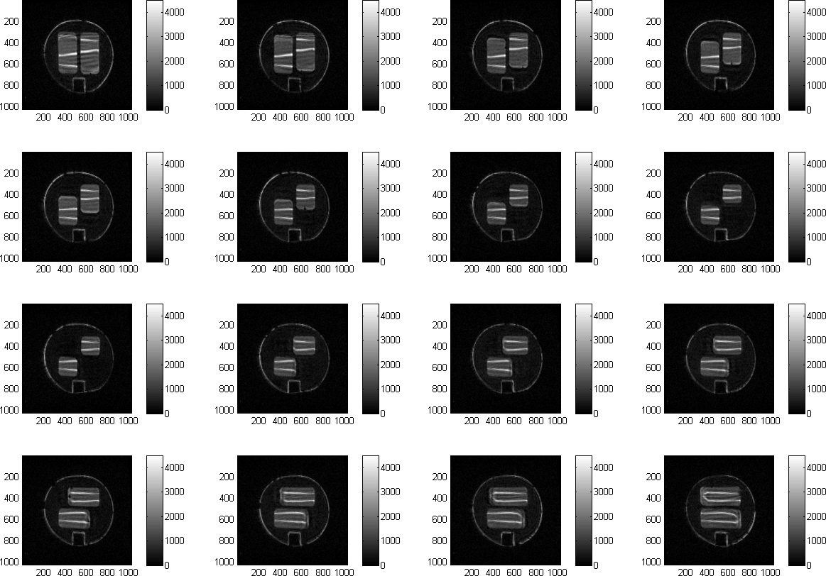
Sequential images through the second mixing section are shown in Fig. 12.

Table 1. Cross sectional area of each plate and average velocity through the cross section, with corresponding Reynolds number (Re); defined for a power law fluid (PL), using an equivalent diameter.

Figure 1. Photograph to illustrate flow through a split-and-recombine mixer using Carbopol dyed red as the minor component and undyed Carbopol solution as the major component.

Figure 2. 2 Tesla super conducting magnet; for size reference, the conveyor is moving 3 avocados into the imaging region.

Figure 3. Plate types and letter designations that are used to create a repeating unit in the SAR mixer.

Figure 4. Schematic of the spilt-and-recombine mixer.

Figure 5. 1 Tesla permanent-magnet-based imaging spectrometer (Aspect Imaging).

Figure 6. Schematic of flow system.

Figure 7. Apparent viscosity of the 0.2% Carbopol solution.

Figure 8. Viscoelastic properties of the 0.2% Carbopol solution.

Figure 9. Repeating units of the SAR mixer.

Figure 10. Two images at the injector: the upstream section of the nozzle has a circular cross section for the doped fluid which gradually becomes a slit at the entrance to the first repeating unit of the SAR mixer.

Figure 11. Fluid downstream of first, second, and third mixing sections, illustrated at Plate H.

Figure 12. Sequences of 16 sequential images through the second mixing section. Please click here to see a larger version of figure 12.

Discussion

Magnetic resonance imaging is a rapid and quantitative method for analysis of fluid mixing. The measurement requires a few minutes to make and provides concentration of fluid as a function of position in the split-and-recombine mixer. This technique is suitable for application to a wide range of mixing problems and geometries [6-11]. Limitations to the technique are that a nonmagnetic mixer must be constructed and used in the MRI equipment, and at least one of the materials must provide a sufficient signal for data acquisition. A sufficient signal requires an NMR active nuclei with a sufficient number density.

MRI can also be used to quantify mixing of solids and liquids, two liquids with significantly different rheological properties as well as mixing in reacting systems. The mixing of solids into a liquid will yield different images than those of the SAR mixer. In the mixing of solids the solid component signal decays rapidly and is not imaged; hence, the signal is from the liquid only and the concentration of solid is derived from the signal loss compared to pure liquid signal.

MRI mixing images provide an excellent test of computational mixing experiments. The image data provides insight on the importance of fluid rheological properties and deviations from ideal conditions. In Fig. 12 the deviations from ideally uniform layers of fluid are evident. The images obtained thus provide detailed data sets suitable for direct comparison with numerical predictions of complex flows.

Materials

Name	Company	Catalog Number	Comments
Aspect 1T imaging spectrometer	Aspect Imaging
AR-G2 rheometer	TA Instruments
Seepex metering pumps	Seepex GmbH
Carbopol	The Lubrizol corporation, (Wickliffe, OH)
Manganese Chloride 1M Solution	Fisher Scientific

References

- Callaghan, P. T. Principles of Nuclear Magnetic Resonance Microscopy. , Clarendon Press. Oxford. (1991).
- McCarthy, M. J. Magnetic Resonance Imaging in Foods. , Chapman & Hall. New York, NY. (1994).
- Mixer. US patent. Sluijters, R. , 3182965 (1965).
- van der Hoeven, J. C., Wimberger-Friedl, R., Meijer, H. E. H. Homogeneity of multilayers produced with a static mixer. Polymer. Eng. Sci. 41, 32-42 (2001).
- Steffe, J. F. Rheological Methods in Food Process Engineering. , 2nd Ed, Freeman Press. East Lansing, MI. (1996).
- Lee, Y., McCarthy, M. J., McCarthy, K. L. Extent of mixing in a two-component batch system measured using MRI. J. Food. Eng. 50, 167-174 (2001).
- McCarthy, K. L., Lee, Y., Green, J., McCarthy, M. J. Magnetic resonance imaging as a sensor system for multiphase mixing. Applied Magnetic Resonance. 22, 213-222 (2002).
- Choi, Y. J., McCarthy, M. J., McCarthy, K. L. MRI for process analysis: Co-rotating twin screw extruder. Journal of Process Analytical Chemistry. 9, 72-84 (2004).
- Rees, A. C., Davidson, J. F., Dennis, J. S., Fennell, P. S., Gladden, L. F., Hayhurst, A. N., Mantle, M. D., Muller, C. R., Sederman, A. J. The nature of the flow just above the perforated plate distributor of a gas-fluidised bed, as imaged using magnetic resonance. Chemical Eng. Sci. 61, 6002-6015 (2006).
- Stevenson, R., Harrison, S. T. L., Mantle, M. D., Sederman, A. J., Moraczewski, T. L., Johns, M. L. Analysis of partial suspension in stirred mixing cells using both MRI and ERT. Chem. Eng. Sci. 65, 1385-1393 (2010).
- Benson, M. J., Elkins, C. J., Mobley, P. D., Alley, M. T., Eaton, J. K. Three-dimensional concentration field measurements in a mixing layer using magnetic resonance imaging. Exp. Fluids. 49, 43-55 (2010).