Waste Water Derived Electroactive Microbial Biofilms: Growth, Maintenance, and Basic Characterization

Summary

Chronoamperometric growth of anodic electroactive microbial biofilms in a fed-batch reactor using a three-electrode setup, controlled by a potentiostat, is demonstrated. The extracellular electron transfer is characterized using cyclic voltammetry in the presence of the electron donor and in the absence of the electron donor. Fundamental data analysis is demonstrated.

Abstract

The growth of anodic electroactive microbial biofilms from waste water inocula in a fed-batch reactor is demonstrated using a three-electrode setup controlled by a potentiostat. Thereby the use of potentiostats allows an exact adjustment of the electrode potential and ensures reproducible microbial culturing conditions. During growth the current production is monitored using chronoamperometry (CA). Based on these data the maximum current density (j_max) and the coulombic efficiency (CE) are discussed as measures for characterization of the bioelectrocatalytic performance. Cyclic voltammetry (CV), a nondestructive, i.e. noninvasive, method, is used to study the extracellular electron transfer (EET) of electroactive bacteria. CV measurements are performed on anodic biofilm electrodes in the presence of the microbial substrate, i.e. turnover conditions, and in the absence of the substrate, i.e. nonturnover conditions, using different scan rates. Subsequently, data analysis is exemplified and fundamental thermodynamic parameters of the microbial EET are derived and explained: peak potential (E_p), peak current density (j_p), formal potential (E^f) and peak separation (ΔE_p). Additionally the limits of the method and the state-of the art data analysis are addressed. Thereby this video-article shall provide a guide for the basic experimental steps and the fundamental data analysis.

Introduction

The elucidation of the fundamentals of microbial extracellular electron transfer (EET) and its exploitation in engineered systems is a vital and rapidly increasing field of research and development^1-3. The study of these electroactive (or bioelectrocatalytic or electrochemically active) microorganisms, including pure strains as well as defined co-cultures and complex consortia, requires a complex arsenal of techniques, methods and protocols⁴. These methods derive from diverse scientific disciplines, e.g. electrochemistry, materials science, microbiology, and provide insights on different hierarchical levels, i.e. from the entire microbial biofilm to single molecules. Thereby, electrochemistry and electrochemical methods represent the fundament of all activities.

Traditionally, fuel cell type setups were often used for the growth and maintenance of electroactive microbial cultures in the archetype of these engineered systems: microbial fuel cells (MFCs)⁵. Unfortunately, these types of MFCs often did not allow monitoring or even controlling the potential of a single electrode and thus, only limited insights in the electrode processes were possible- only the cell voltage was reported. Now it is more and more acknowledged that the individual monitoring and control of the potentials of single electrodes in MFCs represent a clear advantage, not only for fundamental research but also for engineering. Furthermore, with the diversification of the applications of microbial electrochemical technologies that now include, e.g. remediation, desalination, syntheses, and even biocomputing, in so-called microbial bioelectrochemical systems (BES)^2,6,7 an external control of individual electrode potentials is often substantial. This control is usually achieved by using external power sources or potentiostats. Thereby the use of potentiostats allows- in contrast to other types of setups- an exact adjustment of the individual electrode potential. This is of high importance as the electrode represents the terminal microbial electron acceptor (for anodes) or electron donor (for cathodes) of the extracellular electron transfer. Figure 1 depicts the current state of knowledge on the microbial EET at anodes- see for details e.g.^2,4,6,8,9 The EET at the cathode is still mainly untapped¹⁰.

Thus the control of the electrode potential enables not only the use of a reproducible microbial culturing conditions but also its tailoring in terms of EET thermodynamics¹¹. Within this article it is demonstrated how the characteristic parameters of electroactive microbial biofilms can be extracted from fed-batch reactor experiments using chronoamperometry (CA) and cyclic voltammetry (CV). This includes the performance parameters maximum current density (j_max) and coulombic efficiency (CE) as well as EET characteristics. Here the identification of the formal potentials (E^f) of possible and actual electron transfer sites will be in focus. The extraction of these parameters is shown on the example of waste water derived mixed culture biofilms that are dominated by Geobacter spec.¹² These waste water derived biofilms are gained by a simple electrochemical selection procedure as demonstrated by numerous research groups around the world^13-16.

Dynamic electrochemical techniques to study microbial extracellular electron transfer

For a thermodynamic characterization of the EET of electroactive microbial cultures dynamic electrochemical techniques are needed. In general these techniques include potential controlled, i.e. voltammetric, and current controlled, i.e. galvanodynamic, techniques¹⁷. Thereby the potential controlled techniques are more prevalent and include for instance, square wave voltammetry and linear sweep voltammetry¹⁸. Most popular, however, is cyclic voltammetry (CV)^19,20. CV is well-known and widespread in different fields of electrochemistry ranging from battery research via materials science to enzyme bioelectrochemistry²¹. Its application to living microbial cells can only be dated back more than one decade²² and increases significantly during the last years^23,24. Especially the combination of CV and spectroscopic methods has provided unprecedented insights in the EET mechanisms and its molecular nature, e.g.^25,26 In parallel the theoretical framework for the extraction of thermodynamic and theoretical characteristics of the microbial EET was broadened and deepened^27-30. In contrast, however, experimental mishandling or inadequate data-analysis often hamper the appropriate application of CV in the field of microbial bioelectrochemistry. Therefore, in addition to workshops (e.g. at the EU-ISMET 2012) and tutorials¹⁹, this video-article shall provide a basic guide for the conduction of cyclic voltammetric experiments on electroactive bacteria. Thereby it is focusing on the basic experimental steps and the fundamental data analysis and is not intended to provide the latest protocols of kinetic analysis. The most important termini for the following discussion are summarized in Box 1 (adapted from Harnisch and Freguia¹⁹ and modified).

Protocol

As the selection procedure in the bioelectrochemical fed-batch reactor is very specific due to the choice of substrate and anoxic conditions, working in sterile conditions is not necessary for the demonstrated example.

1. Preparation of Growth Medium

1. Prepare a suitable amount of the growth medium by using a phosphate buffer according to Kim et al.¹³ (see Table 1). Here, sodium acetate (10 mM) is serving as substrate. The growth medium used in this article is only one example, and depending on the experimental purpose can vary in its components.
2. Add 1 ml of primary waste water per 20 ml of growth medium as inoculum. The waste water sample is taken from a municipal waste water treatment plant after the mechanical filtration (see for example Figure 2) and can be stored up to three months until usage in a closed container at 4 °C.
   (Note: Depending on the objective of the experiment the exact initial cell count can be important and then should be determined. In the demonstrated example, the initial cell count is not important, as the biofilm reaches steady-state conditions.)
3. Flush the medium including the inoculum with nitrogen for at least 30 min to deaerate it, by inserting a needle in the medium and turn on the nitrogen stream.  The stream should be strong enough that you can observe a complete mixing of the medium.
   (Note: Depending on the volume of the medium one should even consider extending the time of deaeration. During deaeration setup the fed-batch reactor (steps 2.1-2.2))

2. Setup of Fed-batch Reactor

1. Take a suitable reactor vessel- here a modified 4-necked 250 ml round-bottom flask is used.
   (Note: In general the vessel should have at least four inlets. These are necessary for the three electrodes and for sampling/ media exchange. Produced gas volumes can be neglected when the reactor is opened regularly due to sampling or medium change, alternatively a bubble counter should be installed. In order to avoid unwanted phototropic growth, the reactors should be shielded from direct light exposure.)
2. For the three-electrode setup (see Figure 3 and section 3 for details) place the reference electrode (RE) (here Ag/AgCl, sat. KCl, 0.197 V vs. SHE), the working electrode (WE) and the counter electrode (CE) in the flask through individual inlets via silicone plugs – seal air-tight.
   (Note: As WE and CE graphite rods are used. The wire of the electrodes is pulled through the silicon plug and fixed externally. The reference electrode is put through the silicon plug via a drilled hole. To avoid short-circuits, make sure that there is no physical contact of the electrodes, even while stirring or media recirculation. Place the electrodes that they are completely covered with medium solution. For sealing, wrap the silicon plug of every inlet with Parafilm.)
3. Pour the growth medium including the inoculum (here 250 ml) through the sampling port into the reactor while flushing with nitrogen.
4. Close the last inlet with a silicone plug and seal it air-tight. Note: Traces of oxygen will not harm the mixed species biofilms. They are able to withstand and even consume low levels of oxygen which in turn may decrease the CE.

3. Chronoamperometric Biofilm Growth

1. Connect the electrodes to the respective cables of the potentiostat. Place the vessel in a temperature controlled chamber, here 35 °C is used³¹, in order to ensure constant environmental conditions.
2. Open the software to control the potentiostat and choose the technique: Chronoamperometry. Set the parameters for example as follows: A constant potential E_WE of 0.2 V (vs. Ag/AgCl) for a duration t of 500 hr (≈ 20 days). The current is recorded in time steps dt_i every minute.
   Note: The choice of the applied potential is dependent on the studied system/ microorganism. Generally anode processes are studied at positive potential and cathode processes at negative potentials. One can also deduce a suitable potential from the standard potentials of the electron donor/ acceptor and formal potential of the expected microbial electron transfer site, here as a starting point, please refer to recent literature.
3. Start the chronoamperometry. A graph of the measured current over time is plotted by the software, the observed maximum current (i_max) is an important online parameter, as discussed in sections 4 and 5. 

4. Biofilm Maintenance

1. Depending on the environmental conditions, e.g. the temperature, an oxidative current is starting to flow and reaches a plateau (see Figure 4). After reaching zero current again, pause the chronoamperometric measurement and replenish the medium solution. For a faster biofilm growth, replace the medium right after the plateau of the maximum current is reached. Open the sampling port and carefully, without destroying the thin biofilm, discharge the medium. While refilling the medium flush again with nitrogen. Close the sampling port and seal air-tight.
2. Repeat the procedure of step 4.1. until the maximum oxidative current reaches a steady-state (see Figure 4).
   (Note: A constant i_max is believed to indicate a stable steady-state biofilm formation.)
3. Take 1 ml samples of the fresh and the exchanged medium solutions for substrate analysis, e.g. by HPLC. The initial substrate (acetate) concentration (c₀) as well as the concentration of the remaining substrate solution (c₁) are subsequently needed for efficiency calculations (see section Data analysis).
   Note: To achieve unaltered results, e.g. due to further substrate consumption, analyze the substrate samples immediately. If this is not possible, store the samples in a freezer at minimum -18 °C for not longer than a month.)

5. Application of Cyclic Voltammetry to Study EET

1. Perform cyclic voltammetry at the maxima and minima of the current flow as indicated (Figure 4). Depending on the question of interest the CV usually is performed when the system has reached steady-state to get comparable results. (Note: The generation of current is termed turnover conditions and related to the microbial oxidation of the substrate and subsequent electron transfer: microbial bioelectrocatalysis; whereas the nonturnover CVs are performed at (nearly) zero current flow in the CA.)
2. Choose in the potentiostat controlling software the technique: Cyclic voltammetry, and set the appropriate parameters, here for instance: An initial potential of the E_WE to E_i of -0.5 V vs. RE with a scan rate v=dE/dt of 1 mV/sec to a vertex potential E₁ of 0.3 V vs. RE and back to the starting potential E₂ = E_i of -0.5 V.
   Note: When using cyclic voltammetry the applied voltage at the WE is changed linearly with time by the potentiostat (see Figure 5)- Box 2 provides principle rules for choosing the experiment parameters and troubleshooting).
3. Start the cyclic voltammetry and record as many cycles as needed to perform a reproducible CV. Usually, at least 3 cycles are needed.  The resulting plot is called a cyclic voltammogram (see also Figure 7). Note: Depending on the measurement conditions, different information can be gained as demonstrated in the next section.

6. Data Plotting

Here only the plotting of the data is discussed. A more detailed treatise follows in the next section.

1. Use appropriate data analysis software, here all data is exported as text and imported as ASCII file.
2. Calculate and use preferentially current densities (j) and not absolute currents (i).
   (Note: However, as different protocols for calculating j do exist, make clear which one was used. Here the current density per geometric, i.e. projected, surface area of the electrode is used.)
3. Chronoamperometry: Plot the measured current density as function of the time.
4. Cyclic voltammetry: Plot the measured current density as function of the potential of the WE E_we.

Results

1. Chronoamperometry

From Chronoamperometric measurements two operational characteristics can be calculated: the maximum current density (j_max), i.e. the maximum electron flow per second, and the coulombic efficiency (CE), i.e. the total current flow in relation to the consumed substrate. Figure 4 shows a typical chronoamperometric biofilm growth curve of several growth cycles using a fed-batch reactor. After the initial lag-phase a first current density maximum commences. Then the current decreases again due to substrate depletion. At (nearly) zero current flow the medium is exchanged as indicated. After this substrate replenishment the current density increases again and the following maximum current density is higher than the first one. After several growth cycles j_max is constant – which indicates a steady-state biofilm formation¹⁴. As the steady state j_max value is depended on several parameters, e.g. electrode material, reactor temperature and biofilm composition, it is often considered as a characteristic of a certain electroactive microbial biofilm/ electrode system. (In case of flow-through reactors not j_max, but the constant steady-state current density is used.) The second operational characteristic is the coulombic efficiency (CE) (Equation 1). That is the number of electrons recorded as electric current flow, Q_p , per fed-batch cycle related to the number of the theoretical maximum number of electrons Q_th, which is calculated from substrate consumption during this cycle.

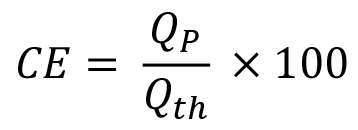
(Equation 1)

The total transferred charge can be gained by integration of the CA curve (see also Figure 6):

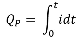
(Equation 2)

The theoretically possible electric charge is calculated by Faraday’s law:

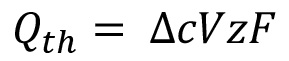
(Equation 3)

Where V is the volume of the growth medium, F the Faraday constant (F = 96,485.34 C/mol), z the released number of electrons of the oxidized substrate (in case of acetate 8 electrons are released during oxidation to CO₂) and Δc = c₀-c₁, which represents the substrate consumption (is determined by chemical analysis methods, e.g. by HPLC).

2. Cyclic voltammetry:

Cyclic voltammograms are recorded for nonturnover conditions and for turnover conditions (as indicated in Figure 4). In both cases different types of information can be gained. In the following it is discussed how possible and actual EET sites can be identified.

2.1 Nonturnover conditions – identifying possible EET sites:

Figure 7 shows typical CVs for nonturnover conditions, i.e. in the absence of substrate. Figure 7A shows the CV of a biofilm for high scan rates (here 50 mV/sec) where only one peak pair and thus one formal potential E^f can be identified. In general the formal potential of a redox couple can be calculated from the peak potential of the oxidation peak E_pA and the reduction peak of the respective species E_pC by forming the arithmetic mean (see also Figure 7C):

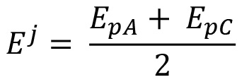
(Equation 4)

When applying a low enough scan rate to the identical biofilm (here 1 mV/sec) up to four redox pairs can be identified (the respective formal potentials are indicated in Figure 7B). The reason is that the capacitive background current is decreased when using lower scan rates, see also Box 1 and e.g.^17,21 for details. However, the nonturnover CV only shows all redox-active compounds at the electrode and thus the E^f of the possible EET sites.  Only the analysis of the turnover CV provides the E^f of the actual EET transfer sites (see step 2.2.).

When further analyzing the nonturnover CVs different other characteristic parameters like peak separation ΔE_p (Equation 5) or maximum peak current i_pA and minimum peak current i_pC can be analyzed (see Figure 7C).

(Equation 5)

These parameters, especially when recorded for different scan rates, can be used for mechanistic and kinetic analysis of electron transfer processes at electrodes. However, this kinetic analysis that is well established for chemical systems is not straightforward for electroactive microbial biofilms, see e.g.^19,30

1. Turnover conditions – identifying actual EET sites:

When performing CV measurement in the presence of substrate a turnover CV is obtained (see Figure 8A). After plotting the data you can see the typical s-shaped, so-called bioelectrocatalytic, curve^17-19. When further analyzing the data, the maximum of the first derivative, i.e. the inflection point of the CV-curve, provides the formal potential E^f of the actual EET site(s) (see Figure 8B). In the case of a young, i.e. thin, Geobacteraceae-dominated biofilm, here 168 h after starting CA, two inflection points can be observed. Subsequently the derivative shows two maxima corresponding to the formal potential of the bioelectrocatalytic active EET sites: -0.376 V and -0.295 V vs. Ag/AgCl (sat. KCl, 0.197 V vs. SHE). In Figure 7B these sites are denominated as E^f,2 and E^f,3, respectively. This finding also shows that the redox processes associated with the formal potentials E^f,1 and E^f,4 (in the nonturnover CV) are not related to bioelectrocatalysis. As the biofilm grows and gets thicker the CV shows only one inflection point, i.e. meaning one maximum in the derivative curve. This formal potential E^f, here being is -0.32 V vs. Ag/AgCl (sat KCl), is (roughly) equal to the arithmetic mean of the two formal potentials assigned to EET of the thin biofilm (e.g. here E^f,2 and E^f,3) – see Figure 9. This shows that this very fundamental CV analysis does provide insights into the EET thermodynamics in a fast and noninvasive way, but noteworthy does not allow drawing further mechanistic or kinetic conclusions.

Notably biofilms gained by the specific conditions in this protocol are highly dominated by Geobacter species (not demonstrated here)^12,15. Changing selected parameters e.g. substrate, temperature, etc. will also influence the microbial composition and thus the electrochemical properties.

Table 1. Growth medium according to Kim et al.³²

Component	(mg/L) / (ml/L)
NaH2PO4•H2O	2,690.00
Na2HPO4	4,330.00
NH4Cl	310.00
KCl	130.00
sodium acetate	820.00
metal solution	12.50
vitamin solution	12.50

Table 2. Components of the metal and vitamin solution33.
Trace element solution:	Vitamin solution:
Component	mg/L	Component	mg/L
Nitriloacetic acid	1,500.0	Biotin	2.0
MgSO4•7H2O	3,000.0	Folic acid	2.0
MnSO4•2H2O	500.0	Pyridoxine hydrochloride	10.0
NaCl	1,000.0	Thiamine hydrochloride	5.0
FeSO4•7H2O	100.0	Riboflavin	5.0
CoSO4 or CoCl2	100.0	Nicotinic acid	5.0
CaCl2•2H2O	100.0	DL-Calcium pantothonate	5.0
ZnSO4	130.0	Vitamin B12	0.1
CuSO4•H2O	10.0	p-Aminobenzoic acid	5.0
AlK(SO4)2	10.0	Lipoic acid	5.0
H3BO3	10.0
Na2MoO4•2H2O	10.0
Note: Dissolve nitriloacetic acid with KOH to pH 6.5, and then proceed to add minerals.

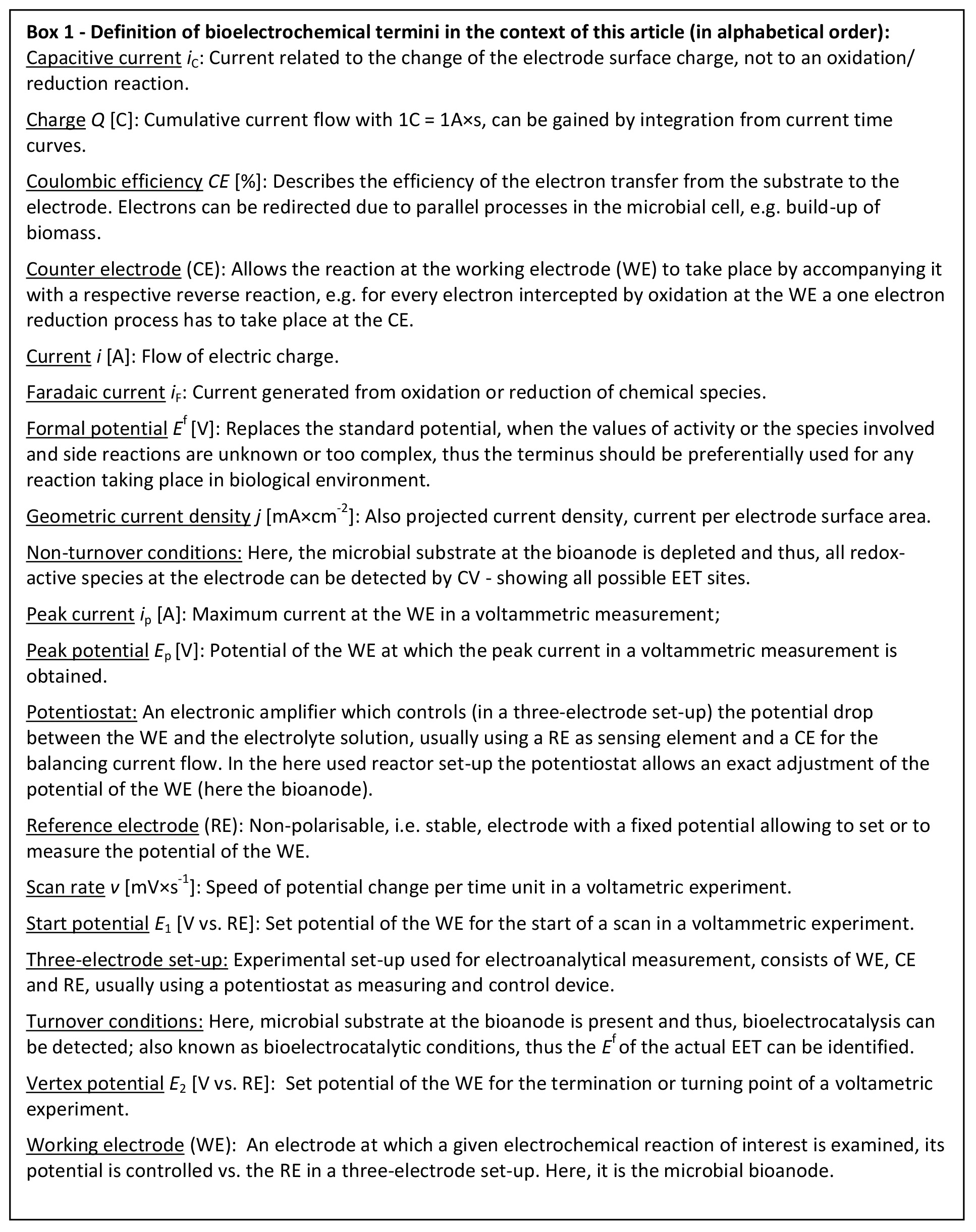
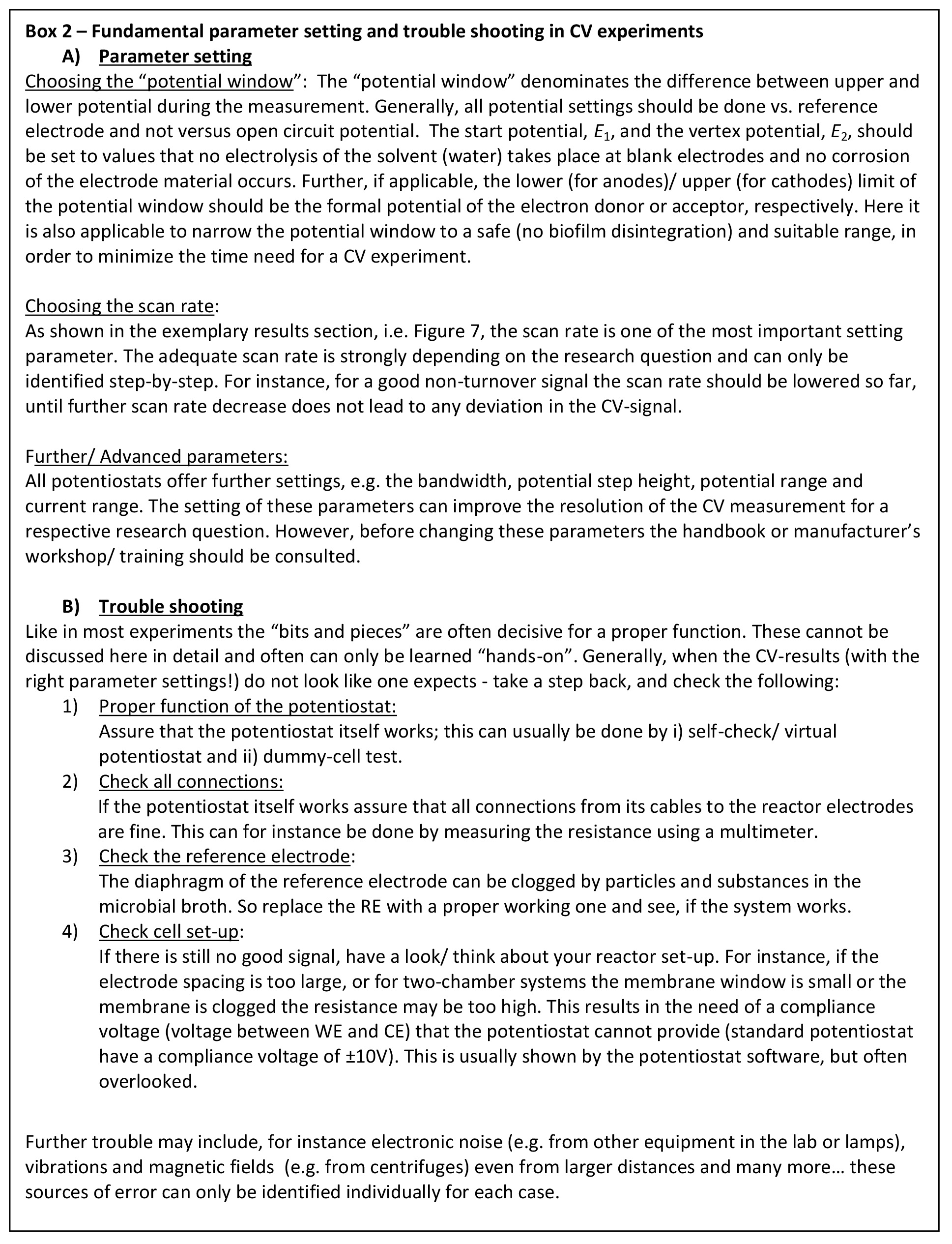
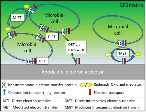
Figure 1. Scheme of possible microbial extracellular electron transfer mechanisms. Click here to view larger image.

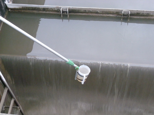
Figure 2. Sampling at the waste water treatment plant after the grid collector (waste water treatment plant Germany). Click here to view larger image.

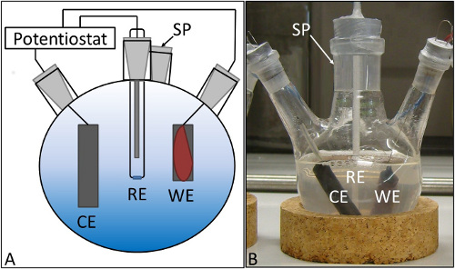
Figure 3. Three electrode setup. (A) Scheme, (B) real reactor; CE = counter electrode, RE = reference electrode, WE = working electrode with electroactive microbial biofilm, SP = sampling port. Click here to view larger image.

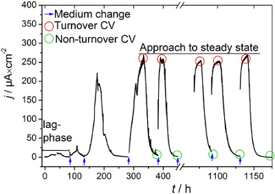
Figure 4. Plot of a chronoamperometric fed-batch waste water inoculum based biofilm growth. The oxidative current reaches a steady-state after three cycles of medium change. Indicated are the lag-phase and the points of time of medium change and conduction of turnover cyclic voltammetry (CV) and nonturnover CV for steady-state biofilm conditions (raw data from Liu¹⁴). Click here to view larger image.

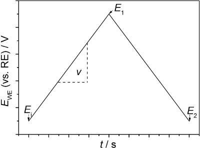
Figure 5. Principle potential-time course during one cycle of cyclic voltammetry. CV is starting at the initial potential E_i. The applied voltage is then changed linearly with time with a scan rate of v. At a chosen vertex potential E₁ the voltage returns to an end potential E₂, here E₂ = E_i. Click here to view larger image.

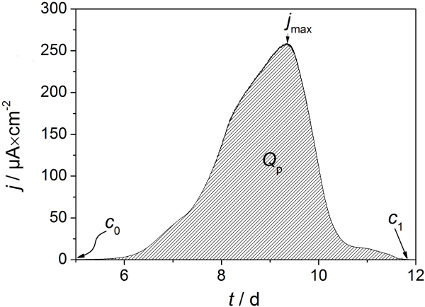
Figure 6. Typical chronoamperogram of one growth cycle of a waste water derived biofilm; herein the maximum current density j_max, the flown (practical) electric charge Q_p, the sampling of the initial substrate concentration c₀ and the substrate concentration after one growth cycle c₁ are indicated. Click here to view larger image.

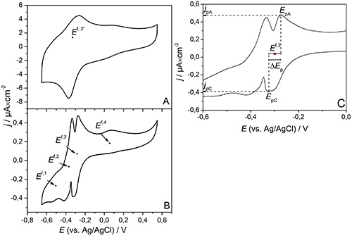
Figure 7. Nonturnover cyclic voltammograms of a G. sulfurreducens biofilm. Scan rate: (A) 50 mV/sec, (B) 1 mV/sec ²³; (C) cutout of B, demonstrating the peak current density (j_pA) and the respective peak potential (E_pA) of the anode at the maxima. Correspondingly at the minima the peak current density (j_pC) and the respective peak potential (E_pC) of the cathode are shown. The formal potential E^f and the peak separation ΔE_p result from Equation 4 and Equation 5, respectively (for details see text below). Click here to view larger image.

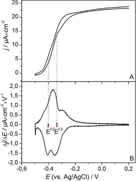
Figure 8. (A) Turnover cyclic voltammogram of a metabolizing G. sulfurreducens biofilm. The scan rate was 5 mV/sec. (B) First derivatives of the voltammetric curve²³. Indicated are the formal potentials of the actual EET sites: E^f,2 and E^f,3. Click here to view larger image.

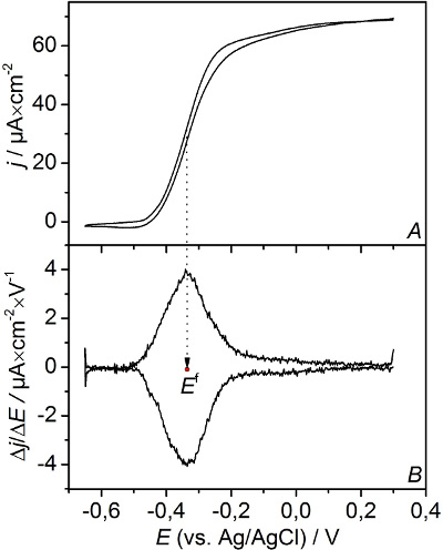
Figure 9. (A) Turnover cyclic voltammogram and (B) first derivatives of a thicker metabolizing G. sulfurreducens biofilm. The scan rate was 5 mV/sec (compare Figure 8). Click here to view larger image.

Discussion

The presented protocol shows an easy and straightforward way for growing electroactive microbial biofilms from waste water inoculate using a three-electrode setup in a fed-batch reactor. Chronoamperometry enables the growth and selection of electroactive microbial biofilms from diverse inocula as well as the fundamental characterization of the biofilms in term of maximum current density and coulombic efficiency. Cyclic voltammetry, being a noninvasive technique, allows performing fundamental studies on the EET thermodynamics of the microbial biofilm and thus to identify possible and actual EET transfer sites. Together, these parameters allow i) characterizing and comparing different microbial biofilms for identical conditions as well as ii) studying the impact of different operational conditions on identical electroactive microbial biofilms. However, these experiments can only be a starting point. On the one hand the multifaceted field of microbial bioelectrochemistry requires further and in-depth exploitation of electrochemical methods and protocols. This includes, for instance, models for extracting kinetic and mechanistic data as well as further methods like electrochemical impedance spectroscopy^34,35. On the other hand electrochemical methods can provide no information on the molecular nature, the microbial composition, the spatial microbial organization, etc. Here further techniques being either noninvasive and coupled to electrochemistry or invasive are needed⁴.  Box 2 provides a short discussion on the critical steps when performing the experiments as well as on initial troubleshooting. 

From the engineering perspective it has to be taken into consideration that the electroactive biofilm anode is only one component of the current microbial bioelectrochemical systems and a multitude of other factors has to be analyzed for full systems³⁶. Yet, we hope that this video-article will help to understand and tailor the core elements of BES, i.e. the microbial electrodes, in future.

Materials

List of materials used in this article

Name	Company	Catalog Number	Comments
Primary waste water	Waste water treatment plant		Taken after mechanical filtration
250 ml Round-bottom flasks with three additional inlets	Th.Geyer Berlin GmbH, Germany	9.011 845	Additional inlets were attached by our in-house glassblower
Ag/AgCl reference electrode (sat. KCl, 0.195 V vs. SHE) with ceramic diaphragm	Sensortechnik Meinsberg, Germany	SE 11
Graphite rods (Ø=1 cm, l=3 and 5 cm)	CP-Handels-GmbH, Wachtberg, Germany		Used as electrode material
Stainless steel, No. 1.4301, Wire Fe/Cr18/Ni10	Goodfellow GmbH, Bad Nauheim, Germany	155-923-05
Silicon plugs	Th.Geyer Berlin GmbH, Germany	9.230 512 and
Parafilm	neoLab, Heidelberg, Germany	3-1011	For sealing to maintain anaerobic conditions
Potentiostat/ Galvanostat Model MPG2	BioLogic Science Instruments, France
EC-Lab	BioLogic Science Instruments, France		software for performing electrochemistry measurements
Origin 8.6	OriginLab		data analysis software

References

- Rabaey, K., Angenent, L., Schröder, U., Keller, J. Integrated Environmental Technology Series. Lens, P. , IWA Publishing. London, New York. (2010).
- Logan, B. E., Rabaey, K. Conversion of wastes into bioelectricity and chemicals using microbial electrochemical technologies. Science. 337, 686-690 (2012).
- Rabaey, K., Rozendal, R. A. Microbial electrosynthesis - revisiting the electrical route for microbial production. Nat. Rev. Microbiol. 8, 706-716 (2010).
- Harnisch, F., Rabaey, K. The Diversity of Techniques to Study Electrochemically Active Biofilms Highlights the Need for Standardization. ChemSusChem. 5, 1027-1038 (2012).
- Logan, B. E., et al. Microbial Fuel Cells: Methodology and Technology. Environ. Sci. Technol. 40, 5181-5192 (2006).
- Harnisch, F., Schröder, U. From MFC to MXC: chemical and biological cathodes and their potential for microbial bioelectrochemical systems. Chem. Soc. Rev. 39, 4433-4448 (2010).
- TerAvest, M. A., Li, Z., Angenent, L. T. Bacteria-based biocomputing with Cellular Computing Circuits to sense, decide, signal, and act. Energy Environ Sci. 4, 4907-4916 (2011).
- Lovley, D. R. Bug juice: harvesting electricity with microorganisms. Nat. Rev. Microbiol. 4, 12 (2006).
- Lovley, D. R. Reach out and touch someone: potential impact of DIET (direct interspecies energy transfer) on anaerobic biogeochemistry, bioremediation, and bioenergy. Rev. Environ. Sci. Biotechnol. 10, 101-105 (2011).
- Rosenbaum, M., Aulenta, F., Villano, M., Angenent, L. T. Cathodes as electron donors for microbial metabolism: Which extracellular electron transfer mechanisms are involved. Bioresource Technol. 102, 324-333 (2011).
- Schröder, U. Anodic electron transfer mechanisms in microbial fuel cells and their energy efficiency. Phys. Chem. Chem. Phys. 9, 2619-2629 (2007).
- Harnisch, F., et al. Revealing the electrochemically driven selection in natural community derived microbial biofilms using flow-cytometry. Energy Environ. Sci. 4, 1265 (2011).
- Kim, J. R., Min, B., Logan, B. E. Evaluation of procedures to acclimate a microbial fuel cell for electricity production. Appl. Microbiol. Biotechnol. 68, 23-30 (2005).
- Liu, Y., Harnisch, F., Fricke, K., Sietmann, R., Schröder, U. Improvement of the anodic bioelectrocatalytic activity of mixed culture biofilms by a simple consecutive electrochemical selection procedure. Biosens. Bioelectron. 24, 1006-1011 (2008).
- Torres, C. sI., et al. Selecting Anode-Respiring Bacteria Based on Anode Potential Phylogenetic, Electrochemical, and Microscopic Characterization. Environ. Sci. Technol. 43, 9519-9524 (2009).
- Virdis, B., Harnisch, F., Batstone, D. J., Rabaey, K., Donose, B. C. Non-invasive characterization of electrochemically active microbial biofilms using confocal Raman microscopy. Energy Environ. Sci. 5, 7017-7024 (2012).
- Scholz, F., Bond, A. M. Electroanalytical Methods: Guide to experiments and applications. 2, edn,(2010).
- Marsili, E., Rollefson, J. B., Baron, D. B., Hozalski, R. M., Bond, D. R. Microbial biofilm voltammetry: direct electrochemical characterization of catalytic electrode-attached biofilms. Appl. Environ. Microbiol. 74, 7329-7337 (2008).
- Harnisch, F., Freguia, S. A Basic Tutorial on Cyclic Voltammetry for the Investigation of Electroactive Microbial Biofilms. Chemistry. 7, 466-475 (2012).
- Marsili, E., et al. Shewanella secretes flavins that mediate extracellular electron transfer. Proc. Natl. Acad. Sci. U.S.A. 105, 3968-3973 (2008).
- Bard, A. J., Inzelt, G., Scholz, F. Electrochemical Dictionary. , Springer. (2008).
- Kim, B. H., et al. Electrochemical activity of an Fe(III)-reducing bacterium, Shewanella putrefaciens IR-1, in the presence of alternative electron acceptors. Biotechnol. Tech. 13, 475-478 (1999).
- Fricke, K., Harnisch, F., Schröder, U. On the use of cyclic voltammetry for the study of anodic electron transfer in microbial fuel cells. Energy Environ. Sci. 1, 144 (2008).
- Marsili, E., Sun, J., Bond, D. R. Voltammetry and Growth Physiology of Geobacter sulfurreducens Biofilms as a Function of Growth Stage and Imposed Electrode Potential. Electroanalysis. 22, 865-874 (2010).
- Busalmen, J. P., Esteve-Núñez, A., Berná, A., Feliu, J. M. C-Type Cytochromes Wire Electricity-Producing Bacteria to Electrodes. Angew. Chem. 120, 4952-4955 (2008).
- Millo, D., et al. In Situ Spectroelectrochemical Investigation of Electrocatalytic Microbial Biofilms by Surface-Enhanced Resonance Raman Spectroscopy. Angew. Chem. Int. Edn. Engl. 50, 2625-2627 (2011).
- Hamelers, H. V., et al. New applications and performance of bioelectrochemical systems. Applied Microbiol. Biotechnol. 85, 1673-1685 (2010).
- Richter, H., et al. Cyclic voltammetry of biofilms of wild type and mutant Geobacter sulfurreducens on fuel cell anodes indicates possible roles of OmcB, OmcZ, type IV pili, and protons in extracellular electron transfer. Energy Environ. Sci.. 2, 506 (2009).
- Torres, C. I., Kato Marcus, A., Rittmann, B. E. Proton transport inside the biofilm limits electrical current generation by anode-respiring bacteria. Biotechnol. Bioeng. 100, 872-881 (2008).
- Torres, C. I., et al. A kinetic perspective on extracellular electron transfer by anode-respiring bacteria. FEMS Microbiol. Rev. 34, 3-17 (2010).
- Patil, S. A., Harnisch, F., Kapadnis, B., Schröder, U. Electroactive mixed culture biofilms in microbial bioelectrochemical systems: The role of temperature for biofilm formation and performance. Biosens. Bioelectron. 26, 803-808 (2010).
- Balch, W. E., Fox, G. E., Magrum, L. J., Woese, C. R., Wolfe, R. S. Methanogens: Reevaluation of a unique biological group. Microbiol. Rev. 43, 260-296 (1979).
- He, Z., Mansfeld, F. Exploring the use of electrochemical impedance spectroscopy (EIS) in microbial fuel cell studies. Energy Environ. Sci. 2, 215-219 (2009).
- Ter Heijne, A., et al. Identifying charge and mass transfer resistances of an oxygen reducing biocathode. Energy Environ. Sci. 4, 5035-5043 (2011).
- Logan, B. Scaling up microbial fuel cells and other bioelectrochemical systems. Appl. Microbiol. Biotechnol. 85, 1665-1671 (2010).
Reprints and Permissions