A Novel Experimental and Analytical Approach to the Multimodal Neural Decoding of Intent During Social Interaction in Freely-behaving Human Infants

Summary

This protocol presents a novel methodology for the neural decoding of intent from freely-behaving infants during unscripted social interaction with an actor. Neural activity is acquired using non-invasive high-density active scalp electroencephalography (EEG). Kinematic data is collected with inertial measurement units and supplemented with synchronized video recording.

Abstract

Understanding typical and atypical development remains one of the fundamental questions in developmental human neuroscience. Traditionally, experimental paradigms and analysis tools have been limited to constrained laboratory tasks and contexts due to technical limitations imposed by the available set of measuring and analysis techniques and the age of the subjects. These limitations severely limit the study of developmental neural dynamics and associated neural networks engaged in cognition, perception and action in infants performing “in action and in context”. This protocol presents a novel approach to study infants and young children as they freely organize their own behavior, and its consequences in a complex, partly unpredictable and highly dynamic environment. The proposed methodology integrates synchronized high-density active scalp electroencephalography (EEG), inertial measurement units (IMUs), video recording and behavioral analysis to capture brain activity and movement non-invasively in freely-behaving infants. This setup allows for the study of neural network dynamics in the developing brain, in action and context, as these networks are recruited during goal-oriented, exploration and social interaction tasks.

Introduction

One of the fundamental human capabilities is the ability to learn and deploy actions (action production) strategically in service of goals and rewards, the ability to apprehend the goals of social partners (action understanding) in order to produce appropriate social responses, and the ability to learn from others through observation and imitation ¹. The neural basis of these cognitive-motor capabilities have been attributed, at least in part, to the so-called mirror neuron system; a system that is thought to be engaged when one views someone performing an action and when one performs the action. However, the potential link between the mirror neuron system and action understanding is not yet well understood ¹. Studying the emergence and development of this mirror neuron system in human infants has been hampered by a) the technical limitations of multi-modal data acquisition of brain activity correlated to intent and fine-grained motion data, b) the constraints imposed by experimental protocols that are unnatural (e.g., social interaction with an agent depicted in a videotape, the need for maintaining a still posture to minimize artifacts during Electroencephalographic (EEG) recordings, etc.), and c) the communication/language barriers when testing young infants/toddlers that greatly limit the researcher’s capabilities to give instructions and validate behaviors.

For a better understanding of the varying neural and behavioral dynamics in natural behavior, we developed a novel experimental and analytical approach that allows the time-resolved study of the neural substrates of emerging goal-oriented and social behaviors in young children. Specifically, we deployed an EEG based mobile brain imaging (MoBI) approach ² to record brain activity and movement from freely-behaving infants during interaction with an experimenter. Inertial measurement units (IMUs) were used to monitor subject and experimenter’s kinematics.

EEG technology and inertial sensors were used to study neural patterns and activations associated to the infants’ action imitation and goal-oriented behaviors in an unscripted interaction with an experimenter/actor. Actions such as reach-grasp, reach-offer, observe, rest, and explore are all part of the cognitive-motor processes involved in imitation. Furthermore, we use source estimation to localize the generators of electric potentials within the brain during the behavioral tasks, thereby studying the spatiotemporal dynamics of neuronal currents throughout the brain. Similarly we deploy machine learning algorithms to assess and measure the predictability of these behavioral actions by identifying action-relevant spatio-temporal patterns in the neural activity in sensor (EEG) and/or source spaces. Integrating traditional ERD/ERS, source and decoding analysis provide a more comprehensive developmental description of the neural basis of such behaviors.

This setup allowed us to exploit the advantages of the MoBI approach ^2,3 and study the social interactions between the infant and the experimenter as they naturally occur without restrictions.

The protocol, from the time the subject arrives to the time he/she leaves, takes approximately 1 hr to complete. The IMU/EEG setup time and electrode location acquisition varies from 15 - 25 min depending on factors such as hair length and cooperation of the subject. The initialization and configuration of the equipment adds up to 10 min, and the testing session lasts approximately 15 min. Removal of the IMUs and EEG cap, including cleaning the head of the infant from the hypoallergenic gel, takes 5-10 min.

Protocol

The following protocol was examined and approved by the Institutional Review Board at the University of Houston. All infant subjects’ parents or guardians received, read, and signed a consent form prior to participation. Parents received free parking and a $20 gift card as compensation for their participation in the study whereas the infants chose an age-appropriate toy.

The recruited infant subjects met the following criteria: 1) Age between 6 and 24 months. 2) Infant was healthy, had normal growth and development, and had no history of natal issues, concussions, seizures, strokes, or learning disabilities. Examples of some common developmental disabilities that would exclude an infant from testing are failure to thrive, undernourishment, and use of alcohol or drugs by the mother during pregnancy.

A simplified flow diagram for the simultaneous recording of multimodal neural activity via scalp EEG and IMUs in freely behaving infants is presented in Figure 1.

1. Informed Consent

1. Show parents the experimental room and briefly explain the purpose of the experiment to them.

2. Scalp EEG Preparation

1. Note: The EEG system used (Table 1) consists of an active electrode system with removable electrodes. Impedance levels are indicated on the electrodes using LEDs.
2. Measure the infant’s head circumference in cm. Place a measuring tape around the widest part of the head, passing it over the eyebrows and around the occipital prominence in the back of the head.
   Note: Measuring the head circumference is necessary for selecting an appropriately sized EEG cap. There are special sizes for the infant population described in Table 1.
3. Place electrodes on an appropriately sized EEG cap (Table 1) as specified by the 10-20 international system. The cap ensures proper placement of the electrodes on the scalp.
   Note: It is preferable to have the cap ready by the time the infant arrives to the study location. Information about the head size can be obtained from the parents before time, or approximated using tables available online [http://www.cdc.gov/growthcharts/html_charts/hcageinf.htm]. If the head measurement does not correspond to the researcher’s approximation, a new cap must be prepared. If multiple caps and electrodes are available, multiple caps can be set up in advance to minimize preparation time.
4. Explain the gelling procedure to the parent. Show them the blunt needle and syringe used to apply gel to each electrode and let them feel the needle on their skin. Use a demo EEG electrode and scalp cap to go over the gelling procedure.
5. Measure the distance from the nasion to the inion along the midsagittal plane of the surface of the scalp. Proceed to fit the scalp cap from behind the infant.
6. Align the Cz electrode with the vertex of the head. Proceed to align and center the Fp1 and Fp2 electrodes on the forehead at approximately 10% of the distance between the nasion and the inion. Align the scalp cap symmetrically along the midsagittal plane of the head. Make sure mid-electrodes [AFz, Fz, FCz, Cz, CPz, Pz, POz, Oz] are aligned with the nasion and inion. When done, secure the cap by strapping below the chin.
   Note: Distract the infant while he/she is being fitted with the EEG cap. An age appropriate video is commonly used to distract infants during setup.
7.  Connect the reference, ground, and recording electrodes to the control box. Turn on the impedance indicators from the control box. 
8. Starting with ground and reference electrodes, use a small syringe to inject electrolyte gel into the space between the scalp and electrode until the impedance of each electrode measures below 60 kΩ. This is indicated by a yellow or green light on the electrodes. Further details on EEG electrode preparation are available in ⁴.
   Note: During the gelling procedure, the infant might move his/her head for various reasons (curiosity, fear, diverted attention). It is therefore recommended that the second experimenter or parent continues to distract the infant. Use the syringes from behind the infant’s head to avoid the risk of hitting the infant’s face with the needle due to unexpected movement of the subject.
9. Connect the amplifiers to the host PC via a USB port using a fiber-optic to USB converter.
   Note: Figure 2A shows the infant subject setup with the EEG cap and the IMU placement. Notice that the electrode cables and the control box are held up, providing load-free mobility to the subject. Figure 2B displays a topographic view of the EEG cap’s electrode locations following the 10-20 labeling system.

3. IMUs Preparation

1. Open the IMU software. Click on “New” on the graphical interface. 
2. Then click “Configure” in the dialog box to configure IMUs. Set the sampling frequency to 128 Hz.
3. Secure the IMUs on the head, chest, and left and right wrists of the infant.
   Note: See Figure 2A. In parallel, fit the experiment’s wrists with IMUs. Make sure IMUs are secured well to the body to minimize inertial measurement errors.
4. Using straps, place the wrist IMUs on the dorsal side of the wrists. Place the chest IMU on the ventral surface near the center of the chest using a harness.
5. Attach the head IMU to the chin straps of the scalp cap so that it is near the left side of the chin. Position the IMUs so that they face outward, with the LED light oriented up.
   Note: The IMUs each weigh about 22 g, and their small size and light weight are unlikely to impede movement. An additional experimenter may be needed to distract the infant for reasons described in step 2.8.

4. Video Capture and Synchronization of Data Streams

1. Place video camera (18) so that the infant (12), the actor (14), and the LED trigger (13) are all clearly visible. See Figure 4.
   Note: Video recordings are used to allow visual annotation and segmentation of behaviors triggered by the experimenter, as well as confirmation of the beginning and end of the recording session.
2. Connect the trigger input/output enclosure (7) to the EEG (5) and IMUs (4). See Figure 3.
   Note: A custom input/output enclosure (7), shown in Figure 3, was designed for aligning all recorded data streams (EEG, IMUs, and video) and thus use event markers from one recording (such as video) or aid the analysis of another recording (such as EEG or acceleration). This is accomplished by using a single momentary pushbutton that, when depressed, will send an active-low (+V to Ground) trigger pulse to EEG (via a DB-25 parallel port), IMU (via a mini-DIN-6 connector), and video (by illuminating a light-emitting diode (LED) positioned in view of the video camera) recordings simultaneously. A 7404 IC logic invertor chip was used to transform the low-state (Ground) to a high-state (+V) pulse, providing the voltage potential needed to power the LED.
3. Have an experimenter in close proximity to the trigger pushbutton and the data collection computer. The experimenter is in charge of operating the trigger, monitoring the data quality throughout the experiment, and saving the data.

5. Preparation of Testing Environment

1. See Figure 4.

6. Data Collection

1. Record the initial impedance values of the EEG electrodes using the control software by selecting the “Impedance Check” tab, clicking the radio button “Impedance On” (wait about 5 sec for electrode impedance values to stabilize), and clicking the “Save impedance” radio button to save impedances. See Figure 5.
2. No filters are applied during EEG data collection.
3. In the EEG recorder program, click on “Monitor” then “Play” to start recoding EEG data. See Figure 6.
4. In the IMU software, click “Stream” and then “Record” in the dialog box to start recording IMU data. See Figure 7.
5. Apply three triggers (III) to signal the start of the experiment using the pushbutton on the input/output enclosure (7). Let the infant rest for 1 min while recording. This provides initial baseline data.
6. Perform experiment and allow the infant subject take breaks as needed. Each experiment trial consists of a turn-taking task where the actor shows an action to the infant using an object (usually, but not always, a toy), passes it to the infant in an effort to initiate an imitation response, and finally retrieves the object back from the infant.
   Note: This exchange is generally repeated for 4-5 trials or until the infant shows no further interest in the object.
7. Given the environment of the session, annotate all timings of each behavior after data collection using the video recording.
8. Record the final impedance values of the EEG electrodes. See step 6.1.
9. Digitize the 3D spatial coordinates of the EEG electrodes using the EEG electrode 3D scanner and software and its corresponding software.
10. Start the 3D scanning software. Go to “File” and select “new workspace”. Load the electrode position file in the first tab of the workspace and provide the necessary information in the storage tab.
11. In the scanning toolbar, click on “start scanning”. Use the 3D scanner, at approximately 30 cm from the infant’s head, to scan the electrode locations by following the changing light patterns on the cap. Once the scanning is complete, the software will automatically save the results.
    Note: At the back of the head, the cables may block the LEDs on the electrodes due to the small size of the infant’s head. The software allows the user to remove some electrodes from the scan without compromising the results. Remove the occipital electrodes from the scan if necessary.

7. Behavioral Segmentation

1. Inspect the video recording of the experiment session and mark the time when the trigger LED blinks (i.e., when the experiment begins and ends), and when any of the previously mentioned behaviors in step 6.6 start and end.

8. Source Imaging

1. Note: Source imaging can accurately identify the generators of EEG potentials within the brain and it usually consists of solving the forward and the inverse problem ⁵.
2. Acquire High resolution T1 weighted Magnetic Resonance Image (MRI) data from public domain databases such as the Neurodevelopmental MRI database which contains average MRI templates as a function of age (in months) for the first two years of life ^6,7.
   Note: This study uses only age-appropriate forward head models of infants and therefore sex information is not taken into account when selecting the MRI template.)
3.  Acquire source volumes for boundary element models (BEM) that include head compartments (i.e., gray matter, white matter, scalp, inner or outer skull) as MRI volumes from the Neurodevelopmental MRI database ⁸.
4. Pre-process BEM MRI volume to obtain a realistic head model by extracting the surface of the brain and head compartments in Curry 7, or similar brain imaging software package.
5.  Import the T1 weighted MRI. Manually identify the three fiducial points such as right/left pre-auricular points and nasion within the brain imaging software, or similar package.
6.  Co-register EEG and MRI space to obtain the rigid geometrical transformation between the MRI‘s space and the subject‘s space by fitting the fiducial points indicated on MRI and the fiducials obtained with 3D scanner in steps 6.9-6.11 using the brain imaging software or similar package.
7. Solve the forward model.
   Note: The forward problem involves the definition of a head model that represents the geometry of the head and of the electrical conductivity properties of the head volume ^9,10.
8. Solve the inverse problem
   Note: The inverse problem tries to infer a location, strength and a time course of a source in the brain from the scalp EEG signals by using signal processing techniques ¹¹.
9. Segment continuous EEG data into trials around the task onset (e.g., imitation, observation segments) with pre- and post-task onset segments of 2 sec length. Identify channels with high impedance as “bad channels” and other artifactual trials in each trial. Pre-process the EEG data for artifact rejection using ICA and reconstruct the bad channels with the average of neighboring artifact-free channels. ^12,13,14.
10. Use the forward model as an input to an automated optimization algorithm that searches over the entire brain to identify the best possible source locations.  
11. Visually analyze the estimated sources and pick up the solutions that most match your expectation based on prior knowledge from the nature of experiment and interpret them carefully.
    Note: This step is the most biased one due to the ill-posed nature of the inverse problem, that is, different configurations of the sources may result in the same surface potentials. Therefore, it may be helpful to perform a sanity check to verify that a given head model and inverse method works well.
12. Perform a sanity check, localizing a known simulated dipole. Namely, for the given head model place a dipole with known configuration, and solve the forward problem to obtain simulated voltages for this dipole.
13. Solve the inverse problem with these voltages on the same head model, to make sure it returns the simulated dipoles.
    Note: These sanity checks should return the dipoles initially placed to a high degree of accuracy.

Results

Figure 8 displays sample EEG and acceleration data from the IMUs for a 16 sec time window recorded during interaction between the subject and the experimenter. EEG data was re-sampled at 100 Hz and then band-pass filtered [1-40 Hz] using a 3rd order, zero-phase Butterworth filter. Channels with high impedance values (Z > 60 kΩ), and peripheral channels, were discarded ^12,15. The IMUs recorded nine signals at 128 Hz: magnetic flux, angular velocity, and linear acceleration in the three Cartesian axes. Here we show the magnitude of the gravity-compensated (GC) acceleration. The effect of acceleration due to gravity was compensated by applying a Kalman filter to predict the IMU orientation in a global frame ¹⁶. Data was segmented by visual inspection of the video recordings (Step 7.1). Vertical solid lines indicate the start of a behavior of interest, as dotted vertical lines represent the ending of the event.

Influence of motion artifacts is present in the EEG data shown in Figure 8 around 709s. The unconstrained approach to data collection in this experimental protocol makes the EEG data susceptible to eye blinks, eye movements, motion and electromyographic artifacts. The data was preprocessed by using a 3^rd order zero-phase Butterworth band-pass filter to constrain it to the delta-band (1-4Hz), and standardized by subtracting the mean and dividing by the standard deviation. High-amplitude artifacts were removed automatically using the Artifact Subspace Removal (ASR) method ¹⁷. Additionally, peripheral channels are excluded from the data analysis in an effort to minimize myoelectric artifact contamination. Frontalis and temporalis muscle contractions merge with EEG signal most prominently at peripheral locations: Frontalis contraction shows up in anterior locations, and temporalis contraction shows up in lateral frontal and temporal locations ¹⁵.

To inspect the nature of the data collected with this protocol, EEG data histograms were plotted in Figure 9. In Figure 9A, it describes the data distribution of the standardized signal from three spatially representative electrodes. The EEG data shows a multimodal distribution for the analyzed behaviors. In Figure 9B the kurtosis values are presented as bar graphs for easier visual inspection of the data.

Classification was performed by extracting time-based lags of each EEG channel, reducing dimensionality while preserving the local scatter of each class (Local Fisher’s discriminant analysis (LFDA)) ¹⁸, and training/testing a model of the reduced set of features (Gaussian Mixture Models (GMMs)) ¹⁹. Training/testing samples were randomly sampled over 20 iterations (i.e., cross-validation) to prevent any over-fitting.Training/testing sample size varies given the number of rejected channels (i.e., impedance greater than 60 kHz), length of experiment session, and number of trials and behaviors expressed. However, the number of training and testing samples used for each class (behavior) correspond to 50% of the least populated class. As an example, the testing set size of each class is N = 1,069 samples for the infant data shown in Figure 10. All pre-processing and classification steps were computed under the MATLAB programming environment.

Figure 11 depicts the whole procedure for EEG source estimation performed in this study in a step-by-step manner. More details about each step is also summarized in section 8.

Figure 12 shows results of event related (de) synchronization (ERD / ERS) in the mu rhythm (5-9 Hz) and the dipole sources during the “Reach-Offer” task. ERS and ERD was calculated as the percentage of a decrease or increase in a frequency-band power which occurs during event (reach and offer task) interval as compared to the reference interval (a segment taken prior to the event). This figure also shows gravity-compensated magnitude acceleration obtained during the task from both wrists of the infant and the actor. For a dipole analysis the EEG signals were decomposed using independent component analysis (ICA) to eliminate background noise. The source estimation was performed in mu rhythm after ICA preprocessing via a fixed MUSIC algorithm ⁵. As expected, the sources were localized over the right primary motor area while the subject was using his left hand to grasp the object.

Product Name	Company	Quantity
BrainAmp Amplifier	Brain Products, Gmbh	2
actiCAP EEG cap- 64 electrodes*	Brain Products, Gmbh	10
actiCAP Control Box	Brain Products, Gmbh	1
Brain Vision Recorder software	Brain Products, Gmbh	1
actiCAP Control Box software	Brain Products, Gmbh	1
CapTrak	Brain Products, Gmbh	1
CapTrak software	Brain Products, Gmbh	1
Opal movement monitor	APDM, Inc	6
Opal docking station	APDM, Inc	6
Opal wireless access point	APDM, Inc	1
Motion Studio software	APDM, Inc	1
Trigger box	Custom	1
Video camera	HC-W850M, Panasonic Co.	1
*The EEG caps come in the following head circumference sizes for infants: 42, 44, 46, 48, 50 cm. For this protocol, a stock of 2 caps of each size is recommended.

Table 1 Equipment.

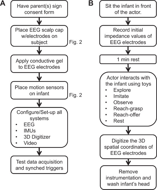
Figure 1. Flow diagrams. (A) Flow diagram of the experiment setup. (B) Flow diagram of the data collection session. Please click here to view a larger version of this figure.

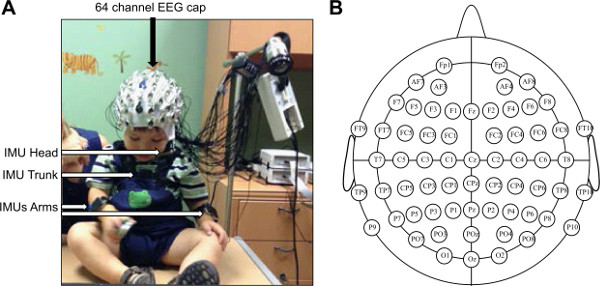
Figure 2. Subject setup and ready for data collection. (A) Frontal view of subject wearing the EEG cap, and four IMUs. (B) Topographic representation of the 64 channel EEG cap using the 10-20 standard electrode positioning system. Please click here to view a larger version of this figure.

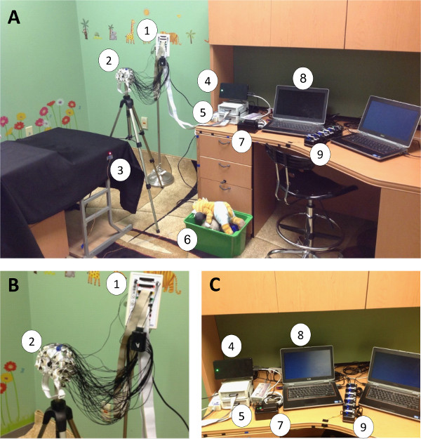
Figure 3. Data collection equipment and the testing room. (A) Data collection equipment setup: EEG control box (1), EEG cap (2), trigger (3), wireless IMU data receiver (4), EEG amplifiers (5), toy box (6), trigger push-button (7), data acquisition laptops (8), IMUs docking station (9). (B) Close-up of EEG cap, active electrodes and control box. (C) Close-up of IMUs and wireless receiver, trigger push-button, EEG amplifiers, and data collection laptops. Please click here to view a larger version of this figure.

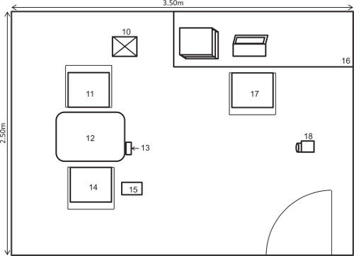
Figure 4. Schematic representation of experimental setting. EEG control box holder (10). Subject’s guardian sits on chair (11), experimenter sits on chair (14) and the person monitoring the data sits on chair (17). The rest of the experimental setup is shown: Interaction tabletop (12), trigger (13), toy box (15), data acquisition table (16), video camera placement (18). Please click here to view a larger version of this figure.

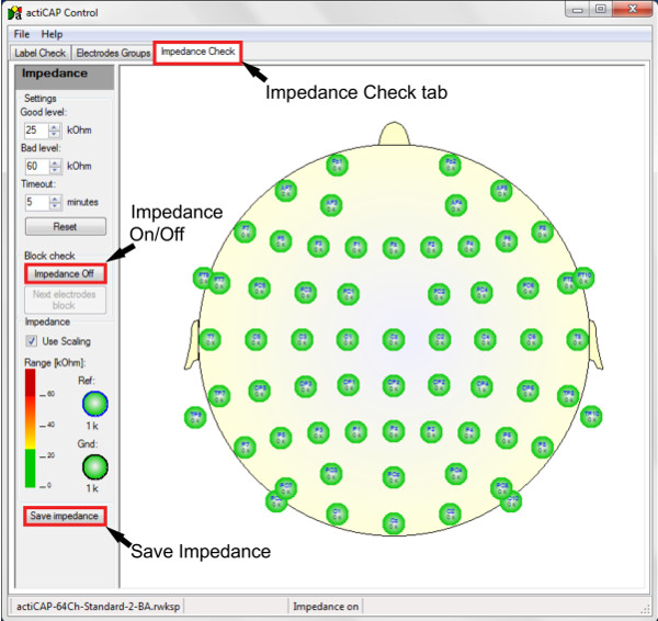
Figure 5. Screenshot of the EEG control software. The arrows point to key icons in the software described in step 6.1 and 6.8. Please click here to view a larger version of this figure.

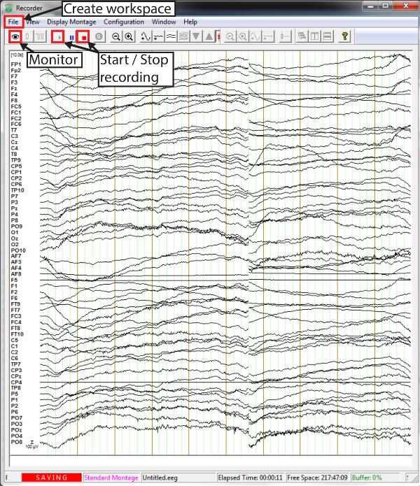
Figure 6. Screenshot of EEG recording software. The arrows point to key icons in the software described in step 6.2 and 6.3. A section of the live-streaming raw data is shown. Please click here to view a larger version of this figure.

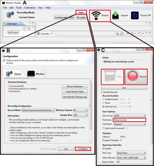
Figure 7. Screenshot of the IMUs software. The red boxes highlight the key icons in the software described in step 6.4. (A) Main command window. (B) Configuration window. (C) Recording window. Please click here to view a larger version of this figure.

Figure 8. Sample data from a representative experimental session. (A) EEG and acceleration data are shown, both band-pass filtered [1-40Hz]. EEG electrodes with low impedance (Z < 60 kΩ) throughout the session are displayed. Solid vertical lines indicate behavior onset. (B) Still frame representations of the infant engaged in the behaviors analyzed: Observe, Reach-grasp, Reach-offer, Imitate, Explore, Rest. Please click here to view a larger version of this figure.

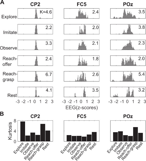
Figure 9. Sample histograms of EEG amplitude for six behaviors identified. A) The data shown corresponds to the raw data from three electrodes (CP2, FC5, POz) recorded in a session with a 20-month old infant. The histograms are scaled to the highest number of occurrences and the kurtosis of each histogram is shown on the right of each plot. Notice the multimodal distribution for most of the behaviors. B) Kurtosis of sample data for each behavior. Please click here to view a larger version of this figure.

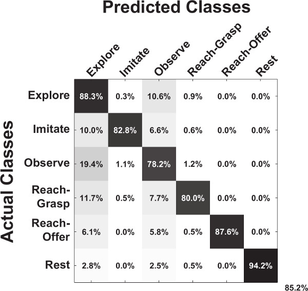
Figure 10. EEG predicts behavioral actions in freely behaving infants ¹². A sample confusion matrix for the classification accuracy for a 20 month old infant is shown. The overall decoding accuracy is displayed on the lower-right corner. Please click here to view a larger version of this figure.

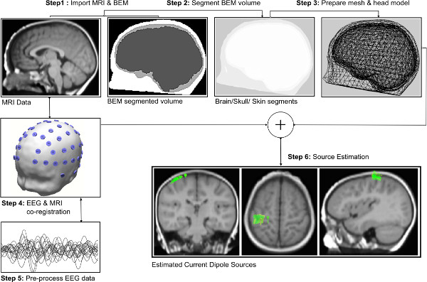
Figure 11. Source Localization. Steps required for an infant dipole source localization using an anatomical MRI and a functional EEG data. Please click here to view a larger version of this figure.

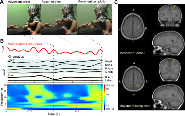
Figure 12. Reach-offer task analysis profile.A) Snapshots of an infant performing the “Reach-Offer” task. B) Mean Global Field Power of EEG in Mu band (5-9 Hz), the limb movement trajectories of the infant and the actor; the grand averaged event related spectral perturbation from all channels. C) Localized dipole sources for two events of “Movement onset” and “Movement Completion”. Please click here to view a larger version of this figure.

Discussion

The protocol described presents a methodology to collect data from freely-behaving infants while they are interacting with an experimenter in real time. It employs mobile brain imaging technology (scalp EEG) to capture neural activity while simultaneously recording kinematic data with IMUs in strategic body locations. The experiment session is also recorded by a video camera. The three data recording systems are synchronized using a custom trigger system.

The EEG and IMU system are strapped to the subject as he/she is freely moving during the experiment session. The IMUs need to be strapped securely to be able to capture kinematics accurately. To ensure full unconstrained mobility of the subject, the equipment has to be as minimally intrusive as possible; thus the use of the holder to support the EEG’s electrode cables and the EEG control box. The experimenter then interacts with the infant for approximately 15 minutes. The infant will elicit an age-dependent repertoire of behaviors during the interaction. These include rest, reach-grasp, reach-offer, explore, observe, and imitate. However, some infants will be unwilling to cooperate in the session due to fatigue, lack of comfort, or stress. Make sure to schedule the experiment when the child is most dynamic and active to prevent the occurence of negative responses from him/her.

The nature of the experiment presents risks to the quality of the data recorded throughout the session. Therefore, it is crucial to test all the connections and data quality before starting the recording session, and to monitor them continuously during the session. If the data EEG system is not recording quality data, stop the software and unplug all connections. Before restarting the software or connecting the equipment back to the laptop, remove all possible noise sources (i.e., power supplies) from the proximity of the recording hardware. The EEG hardware includes signal amplifiers that can pick up environmental noise if placed close to electrical noise sources. For the IMU receiver, make sure there is no interference in the line of sight between the receiver and the experiment and infant.

This experimental setup provides high temporal resolution neural data by measuring electrical activity at the surface of the scalp. Recent studies have demonstrated the feasibility of utilizing these signals, together with whole-body kinematics, to identify classifiable information for expressive movements ²⁰, and functional movements ^21,22, suggesting that this proposed data collection approach could lead to a better understanding of the neural basis of imitation in infants.

Recent contributions featuring powerful machine-learning algorithms applied to brain dynamics ^13,20,21 are building a growing toolkit to study surface potentials in more natural settings. This proposed setup provides a spectrum of possibilities for research questions to be addressed ^2,22. Particularly, it can be applied to research focused on a) understanding the neural basis of cognitive-motor development of infants based on a large population of subjects; b) understanding the neural basis of the baby’s intent in ‘action and context’, which should be predictive of the incoming behavioral action; c) quantifying common and unique neural patterns to characterize individuality and variability in the developing brain; and d) studying the emergence of imitation and learning processes. These goals entail the deployment of machine learning algorithms that can deal with statistically rich data both in informative brain-originated potentials and movement or muscle artifacts ^12,20,23 .

This study attempts to estimate the cortical sources and electric field potentials using the infant EEG data. Due to the technical difficulties such as the lack of knowledge in infant head conductivity values and thickness of cortical matter, the accurate modeling of the head model is a difficult task. Further studies are needed for noninvasive regional tissue conductivity estimates in infants ²⁴. Cortical surface segmentation of infant MRI data presents an additional challenge due to the poor contrast found in images of the developing human brain ²⁵. Future research is needed to address these difficulties and estimate various neurophysiological correlates of infant development and behavior.

Finally, the proposed experimental protocol and methods could be deployed in the study of those with developmental disabilities such as infants with probable autism spectrum disorder (ASD). In such an application, it would be desirable to include a control group and suitable developmental assessments to characterize the two groups (control and ASD). For example, a study group could consist of all high-risk (for ASD) infant siblings assessed with the Autism Diagnostic Observation Schedule ²⁶, symptom severity ²⁷ and the Mullen Scales of Early Learning ²⁸ to characterize general cognitive ability. If available, diffusion-weighted MRI scans would also be highly desirable ²⁹.

Materials

List of materials used in this article

Name	Company	Catalog Number	Comments
BrainAmp Amplifier	Brain Products, Gmbh
actiCAP EEG cap- 64 electrodes*	Brain Products, Gmbh
actiCAP Control Box	Brain Products, Gmbh
Brain Vision Recorder software v1.20.0601	Brain Products, Gmbh
actiCAP Control Box software v1.2.5.2	Brain Products, Gmbh
CapTrak	Brain Products, Gmbh
CapTrak software v1.0.0	Brain Products, Gmbh
Opal movement monitor	APDM, Inc
Opal docking station	APDM, Inc
Opal wireless access point	APDM, Inc
Motion Studio software v1.0.0.201503302222	APDM, Inc
Trigger box	Custom
Video camera	HC-W850M, Panasonic Co.
*The EEG caps come in the following head circumference sizes for infants: 42, 44, 46, 48, 50cm. For this protocol, a stock of 2 caps of each size is recommended.

References

- Woodward, A. L., Gerson, S. A. Mirroring and the development of action understanding. Phil. Trans. R. Soc. B. 369 (1644), (2014).
- Makeig, S., Gramann, K., Jung, T. -P., Sejnowski, T. J., Poizner, H. Linking brain, mind and behavior. Int J Psychophysiol. 73 (2), 95-100 (2009).
- Gramann, K., et al. Cognition in action: imaging brain/body dynamics in mobile humans. Rev. Neurosci. 22 (6), 593-608 (2011).
- GmbH Brain Products. actiCAP Operating Instructions. , Version 006, Author. Munich, Germany. (2013).
- Grech, R., et al. Review on solving the inverse problem in EEG source analysis. J Neuroeng Rehabil. 5 (25), (2008).
- Sanchez, C. E., Richards, J. E., Almli, C. R. Neurodevelopmental MRI brain templates for children from 2 weeks to 4 years of age. Dev Psychobiol. 54 (1), 77-91 (2012).
- Richards, J. E. Neurodevelopmental MRI Database. , Available from: http://jerlab.psych.sc.edu/NeurodevelopmentalMRIDatabase (2010).
- Fuchs, M., Wagner, M., Kastner, J. Boundary element method volume conductor models for EEG source reconstruction. Clin. Neurophysiol. 112, 1400-1407 (2001).
- Song, J., et al. Anatomically Accurate Infant Head Models for EEG Source Localization. J Phys Conf Ser. 434 (1), (2013).
- Roche‐Labarbe, N., et al. High‐resolution electroencephalography and source localization in neonates. Hum Brain Mapp. 29 (2), 167-176 (2008).
- Michel, C. M., et al. EEG source imaging. Clin Neurophysiol. 115 (10), 2195-2222 (2004).
- Hernandez, Z. R., Cruz-Garza, J., Tse, T., Contreras-Vidal, J. L.Decoding of intentional actions from scalp electroencephalography (EEG) in freely-behaving infants. Conf Proc IEEE Eng Med Biol Soc. , 2115-2118 (2014).
- Bulea, T. C., Prasad, S., Kilicarslan, A., Contreras-Vidal, J. L. Sitting and Standing Intention Can be Decoded from Scalp EEG Recorded Prior to Movement Execution. Front Hum Neurosci. , 8(2014).
- Cuevas, K., Cannon, E. N., Yoo, K., Fox, N. A. The infant EEG mu rhythm: methodological considerations and best practices. Developmental Review. 34 (1), 26-43 (2014).
- Goncharova, I. I., McFarland, D. J., Vaughan, T. M., Wolpaw, J. R. EMG contamination of EEG: spectral and topographical characteristics. Clin. Neurophysiol. 114 (9), 1580-1593 (2003).
- Marins, J. L., Yun, X., Bachmann, E. R., McGhee, R. B., Zyda, M. J. An extended Kalman filter for quaternion-based orientation estimation using MARG sensors. Proc. IEEE/RSJ Int. Conf. Intelligent Robots and Systems. 4, 2003-2011 (2001).
- Mullen, T., et al. Real-time modeling and 3D visualization of source dynamics and connectivity using wearable EEG. Conf Proc IEEE Eng Med Biol Soc. , 2184-2197 (2013).
- Sugiyama, M. Dimensionality reduction of multimodal labeled data by local fisher discriminant analysis. J. Mach. Learn. Res. 8, 1027-1061 (2007).
- Li, W., Prasad, S., Fowler, J. E., Bruce, L. M. Locality-preserving dimensionality reduction and classification for hyperspectral image analysis. IEEE Trans. Geosci. Remote Sensing. 50, 1185-1198 (2012).
- Cruz-Garza, J. G., Hernandez, Z. R., Nepaul, S., Bradley, K. K., Contreras-Vidal, J. L. Neural decoding of expressive human movement from scalp electroencephalography (EEG). Front Hum Neurosci. 8 (188), (2014).
- Kilicarslan, A., Prasad, S., Grossman, R. G., Contreras-Vidal, J. L. High accuracy decoding of user intentions using EEG to control a lower-body exoskeleton. Conf Proc IEEE Eng Med Biol Soc. , 5606-5609 (1109).
- Gramann, K., Jung, T. -P., Ferris, D. P., Lin, C. -T., Makeig, S. Toward a new cognitive neuroscience: modeling natural brain dynamics. Front Hum Neurosci. 8 (444), (2014).
- Bulea, T. C., Kilicarslan, A., Ozdemir, R., Paloski, W. H., Contreras-Vidal, J. L. Simultaneous scalp electroencephalography (EEG), electromyography (EMG), and whole-body segmental inertial recording for multi-modal neural decoding. J Vis Exp. 26 (77), (2013).
- Odabaee, M., et al. Neonatal EEG at scalp is focal and implies high skull conductivity in realistic neonatal head models. NeuroImage. 96, 73-80 (2014).
- Knickmeyer, R. C., et al. A structural MRI study of human brain development from birth to 2 years. J Neurosci. 28, 12176-12182 (2008).
- Lord, C., Rutter, M., DiLavore, P. C., Risi, S. Autism Diagnostic Observation Schedule. , Psychological Services. Los Angeles, Calif, Western. (2000).
- Gotham, K., Pickles, A., Lord, C. Standardizing ADO S scores for a measure of severity in autism spectrum disorders. J Autism Dev Disord. 39, 693-705 (2009).
- Mullen, E. M. Mullen Scales of Early Learning. , AGS Edition, AGS Publishing. Circle Pines, Minn. (1995).
- Wolff, J. J., Gu, H., Gerig, G., et al. IBIS Network. Differences in white matter fiber tract development present from 6 to 24 months in infants with autism. Am J Psychiatry. 169 (6), 589-600 (2012).
Reprints and Permissions