Three-dimensional Particle Tracking Velocimetry for Turbulence Applications: Case of a Jet Flow

Summary

A three-dimensional particle tracking velocimetry (3D-PTV) system based on a high-speed camera with a four-view splitter is described here. The technique is applied to a jet flow from a circular pipe in the vicinity of ten diameters downstream at Reynolds number Re ≈ 7,000.

Abstract

3D-PTV is a quantitative flow measurement technique that aims to track the Lagrangian paths of a set of particles in three dimensions using stereoscopic recording of image sequences. The basic components, features, constraints and optimization tips of a 3D-PTV topology consisting of a high-speed camera with a four-view splitter are described and discussed in this article. The technique is applied to the intermediate flow field (5 <x/d <25) of a circular jet at Re ≈ 7,000. Lagrangian flow features and turbulence quantities in an Eulerian frame are estimated around ten diameters downstream of the jet origin and at various radial distances from the jet core. Lagrangian properties include trajectory, velocity and acceleration of selected particles as well as curvature of the flow path, which are obtained from the Frenet-Serret equation. Estimation of the 3D velocity and turbulence fields around the jet core axis at a cross-plane located at ten diameters downstream of the jet is compared with literature, and the power spectrum of the large-scale streamwise velocity motions is obtained at various radial distances from the jet core.

Introduction

Turbulent jet flows are ubiquitous in engineering applications. Detailed characterization of such flows is crucial in a wide spectrum of practical problems spanning from large-scale environmental discharge systems to electronic micro-scale devices. Because of its impact on a number of broad applications, jet flows have been studied in depth^1-4. Several experimental techniques, including hotwire anemometry^4-8, Laser Doppler Velocimetry (LDV)^4,9-12, and Particle Image Velocimetry (PIV)^12-16, have been used to characterize jet flows in a wide range of Reynolds numbers and boundary conditions. Recently, a few studies have been made using 3D-PTV to study the turbulent/non-turbulent interface of jet flows^17,18. 3D-PTV is a technique especially suitable to describe complex turbulent fields from a different perspective. It allows the reconstruction of particle trajectories within a volume in a Lagrangian frame of reference using multi-view stereoscopy. The technique was first introduced by Chang¹⁹ and further developed by Racca and Dewey²⁰. Since then, many improvements have been made on the 3D-PTV algorithm and experimental setup^21-24. With these accomplishments and previous works, the system has been successfully used to study various fluid phenomena such as large-scale fluid motion in a domain of 4 m x 2 m x 2 m²⁵, indoor airflow field²⁶, pulsatile flows²⁷ and aortic blood flow²⁸.

The working principle of a 3D-PTV measurement consists of data acquisition system set-up, recording/pre-processing, calibration, 3D correspondences, temporal tracking and post-processing. An accurate calibration allows for a precise detection of particle positions. The correspondence of the particles detected in more than three image views allows for the reconstruction of a 3D particle position based on the epipolar geometry. A linkage from consecutive image frames result in a temporal tracking that defines the particle trajectories s(t). Optimization of the 3D-PTV system is essential to maximize the likelihood of multi-particle traceability.

First step of the optimization is to acquire an appropriate data acquisition system including high-speed cameras, illumination source and features of seeding particles. The camera resolution along with the size of the interrogation volume defines the pixel size and, therefore, the required seeding particle size, which should be larger than a single pixel. The centroids of detected particles are estimated with sub-pixel accuracy by taking the average position of particle pixels weighted by brightness²¹. The camera's frame rate is closely associated with Reynolds number and the ability to link detected particles. A higher frame rate allows for resolving faster flows or a larger number of particles since the tracking becomes more difficult when the mean displacement between images exceeds the mean separation of the particles.

Shutter speed, aperture and sensitivity are three factors to consider in the image capture. Shutter speed should be fast enough to minimize blurring around a particle, which reduces uncertainty of particle centroid position. Camera aperture should be adjusted to the depth of field of the interrogation volume to reduce the probability of detecting particles outside the volume. Since the maximum sensitivity of a camera is fixed, as the frame rate increases, the necessary light required to illuminate the particles should increase accordingly. Unlike PIV, complex optic settings and high-power lasers are not strictly required in 3D-PTV, as long as the light source is sufficiently scattered from the tracer particles to the camera. Continuous LED or halogen lights are good cost-effective options that bypass the need of synchronization²¹.

In 3D-PTV, like other optical flow measurement techniques, tracer particle velocity is assumed to be the local instantaneous fluid velocity²⁹. However, this is only the case for ideal tracers of null diameter and inertia; tracer particles should be large enough to be captured by a camera. The fidelity of a finite particle can be determined by the Stokes number S_t, i.e. the ratio of the relaxation time scale of particles and the time scale of turbulent structures of interest. In general, S_t should be substantially smaller than 1. For S_t  ≤0.1 flow tracking errors are below 1%³⁰. In-depth discussion can be found in Mei et al.^29-31. Recommended particle size for a 3D-PTV experiment varies depending on the light source and camera sensitivity. With halogen or LED lights as illumination sources, relatively larger particles are used (e.g. 50-200 µm)³², whereas smaller particles (e.g. 1-50 µm)^33,34 can be used with a high power laser (e.g. 80-100 Watts CW laser). Particles with high reflectivity for a given wavelength light, like silver coated under halogen light, can amplify their mark into an image. The seeding density is another important parameter for a successful 3D-PTV measurement. Few particles result in low number of trajectories, while an excessive number of particles cause ambiguities in establishing correspondences and tracking. Ambiguities in establishing correspondences include overlapping particles and detecting multiple candidates along the defined epipolar line. In the tracking process, the ambiguity due to a high seeding density is occurred because of the relatively short mean separation of particles.

Second step is optimal settings in recording/pre-processing to enhance the image quality. Photographic settings, such as gain & black level (G&B), play an important role in optimizing the image quality. Black level defines the brightness level at the darkest part of an image, whereas gain amplifies the brightness of an image. Slight variations of the G&B levels can significantly impact the likelihood of traceability. In fact, high G&B may over-brighten an image and eventually damage the camera sensor. To illustrate this, the impact of G&B levels on the flow reconstruction is also examined in this article. In the pre-processing step, the images are filtered with a high-pass filter to emphasize light scatter from particles. The pixel size and gray scale are adjusted to maximize the particle detection within the interrogation volume.

Third step of the optimization is accurate calibration of the stereoscopic imaging, which is based on epipolar geometry, camera parameters (focal length, principle point, and distortion coefficients), and refractive index changes. This process is essential to minimize the 3D reconstruction error of the fiducial target points. Epipolar geometry uses relative distances (between camera and interrogation volume) and tilted angle from the target image. Refractive index changes along the camera view through the interrogation volume can be taken into account based on the procedure of Mass et al.²¹. In this experiment, a 3D stair-like structure with regularly distributed target points is used as a target.

In a 3D-PTV experiment, although only two images are needed to determine a 3D particle position, typically more cameras are used to reduce ambiguities²¹. An alternative to expensive setups with multiple high-speed cameras is the view splitter, proposed by Hoyer et al.³⁵ for the use of 3D-PTV and recently applied by Gulean et al.²⁸ for the biomedical applications. The view splitter consists of a pyramid-shaped mirror (hereon primary mirror) and four adjustable mirrors (hereon secondary mirror). In this work, a four-view splitter and a single camera were used to mimic the stereoscopic imaging from four cameras. The system is used to characterize the intermediate flow field of a pipe jet with a diameter, d_h = 1 cm and Re ≈ 7,000 from a Lagrangian and Eulerian frames at around 14.5-18.5 diameters downstream from the jet origin.

Protocol

1. Lab Safety

1. Review the safety guidelines of the selected illumination source (e.g. laser, industrial LED, halogen).
   Note: in this experiment, a set of five 250 Watts halogen spotlights are used as illumination. Basic safety and recommendation aspects for this light source are described as follows.
   1. Avoid direct contact with halogen lights, which operate at high temperatures (~3,000 K color temperature).
   2. Keep the light ON only when acquiring data to avoid heating the flow under consideration.
   3. Keep away all burnable materials near the light source, including paper of any kind.

2. Experimental Set-up

1. Choose the Appropriate Lens
   1. Choose a lens with low aberration to avoid calibration problems. Recommended lens types are telephoto or micro lenses.
   2. Make sure that the lens covers the desired field-of-view (FOV) within the object distance, O, by estimating the needed magnification, M.
      Note: the magnification is the ratio of the length of the camera chip to the FOV, and the object distance can be computed as O = f(1/M + 1), where f is the focal length of the lens. In this experiment, the length of the camera chip is 20.34 mm and the corresponding FOV, or the primary mirror, is 50 mm with the limited object distance O ≤250 mm. (The object distance is restrained due to the finite length of the slider where the camera and the view splitter are mounted.) The magnification is M = 20.34/50 = 0.41, and approximate focal length with the given range of the object distance is f ≤72.7 mm. Thus, a micro lenses with a focal length of 60 mm is used with a focal ratio of f/2.8D.
2. Mount and Adjust the Camera with the View Splitter.
   1. Level the center of the primary mirror with that of the interrogation volume by sliding the mirror along the vertical mounting post and fixing the mirror with the post holder. Note that this step is performed before installing the secondary mirrors.
   2. Mount the camera and set the center of image coincident with the center of the primary mirror.
   3. Adjust the width and height of the camera view to just cover the primary mirror by controlling the region of interest (ROI) setting in the recording software. This process is to reduce image size and image noise. Note: in this experiment, the size of the primary mirror is 5 x 5 cm² (1,728 x 1,728 pixels).
   4. Design a (customized) 3D calibration target. It should enclose the whole investigation volume. Ensure that each view of the splitter captures all the target marks to allow a uniform calibration.
      Note: in this demonstration, the target was 3D Printed using vero back plastic. It has a stair-like shape with dimension 35 x 35 x 30 mm³, with 1 mm diameter white target points separated 2.5 mm, 5 mm and 10 mm in the vertical, streamwise and spanwise directions. Accurate geometry of the target is crucial as it projects into a calibration model and position of the cameras with respect to the flume.
3. Place the Calibration Target into the Interrogation Volume.
   1. Position the calibration target on an adjustable height platform facing towards to the camera.
   2. Match the height of the center of the calibration target with the center of the interrogation volume by adjusting the height of the target platform.
      Note: in this example, the center mark of the calibration target is leveled with the center of the jet nozzle, 20 cm height. A bubble level gauge can be used to level the target.
4. Mount and Adjust the Secondary Mirrors of the Four-view Splitter.
   1. Locate the primary mirror at a distance from the interrogation that ensures its full capture. It is 0.2 m for this demonstration (Figure 1).
   2. Mount secondary mirror at its approximate position, where the camera view from each side of the primary mirror is roughly aligned with a secondary mirror. Secure the secondary mirror by fixing it to the secondary mirror's vertical mounting post.
   3. Repeat this process for the other three mirrors. Check geometrical symmetry of all secondary mirrors with respect to the primary mirror.
   4. Make final adjustments by adjusting the mirror mount of the secondary mirrors to ensure that each of the four views encloses the entire calibration target. One efficient way to check the mirrors' positions and angles is to use a laser pointer to visualize each view's image path.
   5. Check for overlapping of sub-images by moving one mirror.
      Note: If only one view changes, then the overlapping region is negligible. Otherwise, repeat steps 2.4.2 to 2.4.5 until the overlapping region is minimized.
5. Place light source(s) directly facing the interrogation volume. Make sure to have the camera covered when adjusting the light to avoid damage on the camera sensor.
   1. Check that the light source is uniformly distributed over the entire investigation volume.
   2. Enhance the light intensity, if necessary, by placing a magnifying lens directly under the light sources. Note: in this experiment, a plano-convex magnifying lens of focal distance f₀ = 450 mm is used to intensify the illumination.

3. Set-up Optimization

1. Turn on and Adjust the Settings on the Camera to increase the Image Quality.
   1. Adjust the lens magnification until the reflection through the primary mirror is equally focused in all four views of the secondary mirrors.
   2. Check that the images from the view splitter are symmetric and capture the interrogation volume by observing the symmetry of the calibration target image from the four views.
   3. Adjust the f-number to capture the closest and the furthest calibration target points from the camera.
      Note: This allows the camera to capture tracer particles only in the depth of the interrogation volume. In this example, the f-number is 11.
   4. Set the desired frame rate as 550 Hz (it depends on particular application, see Introduction) and maximize the light sensitivity accordingly in the recording software.
2. Check illumination in each view of the primary mirror by observing the particle density difference in each view of the splitter through a live camera view.
   Note: If multiple light sources are used to illuminate the interrogation volume, it is probable to have differences in each view of the splitter. In this experiment, the top two secondary mirrors received less light because the illumination comes from the top. The use of a flat mirror at the bottom of the flume can help to reduce the light variation across the views.
3. Turn off the background lights in the room before using 3D-PTV light sources.
4. Adjust the G&B level of the camera to better capture the light scatter from the particles. Record several short sequences with various G&B levels and find the optimum one by observing the distribution and density of particle trajectories.
   Note: in this experiment, the range of G&B level was 0-500, and black (B) level was set to 500, to brighten the dimmer light scatter, whereas, gain (G) was set medium, 300, to moderately amplify image signals and avoid over-brighten the image.

4. Calibration

1. Place the calibration target in the investigation volume before adding tracer particles, and take few calibration images. Use a dimmer light source (e.g. LED flash light) to illuminate the target.
2. Divide the calibration image into four independent sub-images and make a text file containing the reference coordinate positions of the target marks. OpenPTV software (http://www.openptv.net) is used here for this purpose.
   Note: onward processing is identical to users employing a multiple camera set-up.
3. Click 'Create calibration' tab to start the calibration process after saving images and the text file obtained in step 4.2 in the 'Cal' folder of the software.
4. Click the 'Edit calibration parameters' tab and choose the 'Calibration Orientation Parameters' tab to define magnification, rotation angles and distance between the center of each split view and the origin of the calibration target.
   Note: The first row is the distance from the origin calibration target to the camera sensor in the x,y,z direction. The second row indicates the angles, in radians, around the x,y,z axes. Next, a 3 by 3 data represents the rotation matrix. Then, the two following rows are the pinhole distances of the x and y axes from the image center (mm) and focal distance. The last row contains the position of the flume glass in respect to the origin target in the x,y,z direction.
5. Click 'Detection' and 'Show initial guess' to investigate that the 'guess' points are matched with the detected target points.
6. Repeat step 4.4 for all four views until the 'guess' points are aligned with the set of calibration images.
7. Click 'Orientation' to reconstruct the orientation of the interrogation volume.
   Note: The calibration can be improved by adjusting the lens distortion and affine transformation. Now, the investigation volume is calibrated and ready to process data. See author's thesis³⁶ for additional description the calibration process.

5. Flow Setting/Data Collection

1. Estimate the maximum amount of particles captured in each camera view from the frame rate and maximum flow velocity. In this demonstration, the reference velocity is U ≈ 0.4 m/sec, the frame rate is 550 Hz and ~4 x 4 x 4 cm³ interrogation volume. This resulted in ~1,000 particles per frame.
2. Turn on the camera with the optimized settings obtained in step 3.
3. Add seeding particles and wait several mean residence time to allow the flow reaching a steady state. Add more particles if needed but avoid high seeding density, estimated in the step 5.1, which may cause ambiguities.
   Note: in this example, ~1.6 g of 100 m silver-coated hollow ceramic spheres of 1.1 g/cm³ density are used as seeding for the fluid medium (2 x 0.4 x 0.4 m³).
4. Record the desired number of flow images.
   Note: in this experiment, 9,000 images at 550 Hz were captured using the recording software. Repeat steps 2.4 to 5.3 if the camera and/or view splitter is moved (even a slight motion can heavily affect results).

6. Data Processing (Via OpenPTV Software)

1. Divide the raw image obtained in step 5.4 into four independent sub-images.
2. Click 'Init/restart' under the 'Start' tab to load initial images from four views.
3. Right-click the 'Run' directory and click 'Main Parameters' to control number of cameras, refractive indices, particle recognition, number of sequence images, observation volume and criteria for correspondences.
   1. Define the number of cameras (views) used for the experiment under the 'General' tab. In this experiment, set the number of cameras as 4.
   2. Define refractive indices along the camera view under the 'Refractive Indices' tab.
   3. Define the min and max numbers of pixel detection as well as gray value threshold to optimize the number of particle detection in all four views under the 'Particle recognition' tab. The min and max numbers of pixel detection and gray threshold determine the pixel size and brightness level for particle detection. It eliminates noise and particles out of focus.
   4. Define the number of images to process under the 'Parameters for sequence processing'.
   5. Define the observation volume under the 'Observation Volume' tab.
   6. Define the correlation of correspondences under the 'Criteria for correspondences' including total band parameter (mm) for stereo matching.
4. Click 'High pass filter' under the 'Preprocess' tab. This intensifies light scattering from particles in all four views.
5. Click 'Particle Detection' to determine the centroid of detected particles at sub-pixel level for all four views. Repeat steps 6.2 and 6.3 until the number of detected particles similar to the expected number of particles calculated in step 5.1.
6. Click 'Correspondences' to establish stereoscopic correspondences in each view.
   Note: To reconstruct the 3D position of detected particles, correspondences should be determined at least from three views.
7. Click '3D positions' to obtain detected particle 3D position based on the calibration.
8. Click 'Sequence without display' to repeat the process from steps 6.4 to 6.7 for all image sequences.
   Note: This creates a 'rt_is' file for each image set containing a summary of detected particles in the frame with a tab-separated text file format.
9. Right-click the 'Run' directory and click 'Tracking Parameters' to define parameters of radius sphere, (e.g. dvxmin and dvymin in mm/frame), to search candidate particles for tracking.
10. Click 'Tracking without display' to define particle identification (ID) of reconstructed particles obtained in step 6.7.
    Note: It correlates a sequence of adjacent frames for tracking using a four-frame predictor predictor-corrector scheme²⁴. This process creates a ptv_is file for each image set which contains tracking information of detected particles in the frame; the first two columns show the particle ID in the previous frame and in the next frame, respectively.
11. Click 'Show trajectories' to visualize trajectories in each camera view.

7. Post Processing (Optative)

Note: the reach and type of post-processing depends on individual needs and it is, therefore, customizable. Here, point base calculations are briefly described as an example.

1. Obtain Data in Lagrangian Frame (via Matlab).
   1. Extract the 3D position of each particle and its associated ID from the ptv_is files. It allows linking detected particles among image sequences to reconstruct trajectories.
   2. Calculate velocity and acceleration of particles from the given frame rate for each trajectory. In this demonstration, the velocity and acceleration of particles are calculated by low-pass filtering the position signal with a moving cubic spline^34,37.
   3. Make a struct array format with fields containing 3D positions, 3D velocities, 3D accelerations, and time stamp as well as trajectory ID of each trajectory. In this data format, the length of struct array represents number of trajectories.
2. Obtain Data in Eulerian Frame (via Matlab).
   1. Transform the struct array (step 7.1.3) to a temporal one using the time stamp of each particle. This creates a similar struct array structure obtained in step 7.1.3, but the length of struct array now represents the frame numbers, which is 9,000 in this experiment.
   2. Interpolate the temporal struct array into a three dimensional grid for each time frame to obtain instantaneous velocity fields in Eulerian coordinates. In this demonstration, the griddata function in Matlab is used to perform the interpolation.

Representative Results

A photograph and a schematic of the setup are shown in Figures 1 and 2. The calibration target, the fiducial marks reflected on the view-splitter and 3D calibration reconstruction are illustrated in Figure 3. The RMS of the recognized calibration targets is 7.3 µm, 5.7 µm and 141.7 µm in the streamwise x, spanwise y, and depth z directions. The relative higher RMS in the z-coordinate is due to the reduced targets points with respect to those in the other directions and relatively small angles of four views with the z-axis compared to x and y coordinates. The detected particles in each of the four views at any given instant were on the order of 10³. Among the detected particles, the number of successful 3D reconstructions is reduced to roughly half due to the fact that only particles in the intersection region are captured. Video 1 shows a high-speed video sample of the jet flow from the four-view splitter.

A sample of four representative particle trajectories in the intermediate-field region around and crossing the x/d_h=16 plane at radial distances r/d_h=v0, 1.5, 3 from the jet core is illustrated in Figure 4. As expected, longer trajectories in the given time interval (Δt ≈ 1 sec) are observed around the jet core. At the edge of the jet (r/d_h ≥2), tracer particles exhibit short and more complex trajectories. Figure 5 shows all the successfully reconstructed particle trajectories crossing the x/d_h = 16 plane. The particle velocities in the selected domain exhibit a wide distribution ranging from nearly 0 to 0.6U_j, where U_j ≈ 0.6 m/sec is the exit velocity of the jet, and acceleration/deceleration, ∂U⁄∂s, where is the Cartesian coordinate. It also reveals that an substantial portion of the particles within the vicinity of the jet core exhibit smoother trajectories. The particle trajectories, s(t), allows for the estimation of the position, velocity and acceleration. Figure 6a shows the case of a particle crossing the x/d_h = 16 plane around the jet core. Figure 6b, 6c, and 6d show the 3 components of the particle trajectory, velocity and acceleration as a function of normalized time. It is worth highlighting that the local particle acceleration can be several times the standard gravity. The particle trajectories allow for obtaining specific features of the particle trajectories via the so-called Frenet-Serret frame. It describes the changes of the orthonormal vectors (tangential, normal, binormal) along s(t). Of particular relevance is the curvature, κ, which is the inverse of the radius of curvature, ρ, and defined as:

where = dr/ds is the tangent unit vector of the trajectory and r is the position vector (Euclidean space) of the particle as a function of time, which can be written as a function of , i.e., r(s) = r(t(s)). The curvature, κ, is computed for all the particles crossing the x⁄d_h = 16 and x⁄d_h = 17 planes. The mean curvature, , as a function of the distance from the jet core r is calculated as:

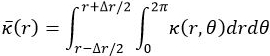
where Δr = 0.2d_h is used in here. Figure 7 illustrates = f(r) normalized by d_h. It shows a relatively low and nearly constant  within the area defined by the circular cross section of the pipe, r/d_h ≤0.5. At a larger distance from the jet core in the x/d_h = 16 plane, increases monotonically. A similar trend is obtained at the x/d_h = 17 plane, but with a reduced  outside the jet core (r/d_h ≥0.5). It is worth highlighting that this flow feature can be inferred only with the 3D-PTV technique. The data quality based on various levels of G&B settings is assessed in terms of the ratio of linked particles to the rest of 3D-reconstructed particles shown in Table 1. The highest link ratio is observed at the G&B setting of 300&500.

Eulerian flow characteristics can be achieved by grid-interpolation, which mimics 3D particle image velocimetry (3D-PIV). It is important to note that due to the comparatively low particles tracked at each time, a significantly higher number of frames are needed to truly mimic PIV quality for an Eulerian description. This is more critical in the estimation of high-order statistics (e.g., turbulence intensity and Reynolds stresses). The streamwise velocity at the jet core for various G&B levels is illustrated in Figure 8. The measurements are compared with the theoretical behavior:

where U₀(x) is the streamwise velocity at the jet core, B ≈ 6 is a constant, and x₀ is the virtual origin³⁸. The figure shows the relevance of setting the G&B levels. Figure 9 illustrates the mean velocity distribution of the jets in the x/d_h = 16 plane.

Finally, the spectral distribution ϕ(f) of the large-scale motions of the streamwise velocity at locations r/d_h = 0, 0.6, and 1 in the x/d_h = 10 plane is illustrated in Figure 10. A Butterworth low-pass filter was applied to the velocity time series with cut-off frequency, f_c = 200 Hz.

Figure 1: Schematic of the experimental set-up. Please click here to view a larger version of this figure.

Figure 2: Experimental set-up. This illustrates various views of the camera and the four-image view splitter, flume and interrogation volume: (top left) top view, (bottom left) back view of the camera and view splitter system, (top middle, bottom middle) side views of the overall experimental set-up, (right) zoom-in view of seeding particles in the jet flows. Please click here to view a larger version of this figure.

Figure 3: Calibration: (a) Calibration target, (b) Image-set of the calibration target from the view splitter, (c) 3D recognition of the fiducial marks from the calibration target. Please click here to view a larger version of this figure.

Figure 4: Selected particle trajectories at r⁄d_h = 0, 1.5, 3. Please click here to view a larger version of this figure.

Figure 5: Particle trajectories crossing the x/d_h = 16 plane, where velocity is shown as a color level. The interrogation volume shown in the figure is contained between (x)⁄d_h (14.5,18.5), y⁄d_h (-2,2), and z⁄d_h (-2,2), where (x, y, z) = (0, 0, 0) is located at the center of the jet origin. The velocity along the individual trajectories, normalized by the bulk velocity U₀, is illustrated as a color level. Please click here to view a larger version of this figure.

Figure 6: (a) Particle trajectory, (b) displacement, (c) velocity, and (d) acceleration of an arbitrary particle. Please click here to view a larger version of this figure.

Figure 7: Curvature of the particles: Graph showing mean curvature of the particles as a function of the radial distance from the jet core at the planes x⁄d_h = 16 and x⁄d_h = 17. Please click here to view a larger version of this figure.

Figure 8: Streamwise velocity at the jet core within (x)⁄d_h (15,18) for various G&B levels. Three G&B levels are included (300&500 (optimum), 300&250, 100&250). Please click here to view a larger version of this figure.

Figure 9: Non-dimensional distribution of the streamwise velocity component at x/d_h = 16. Please click here to view a larger version of this figure.

Figure 10: Power spectrum ϕ(f) of the streamwise velocity component at a point located at r/d_h = 0 (jet core), 0.6, and 1 in the x/d_h = 16 plane. Please click here to view a larger version of this figure.

Video 1: Video sample of the jet flow from the four-view splitter, 10 times slower than actual speed obtained at 550 fps (right click to download).

Table 1: The ratio of linked particles to the rest of 3D-reconstructed particles at various G&B levels. Three G&B levels are included (100&250, 300&250, 300&500).

Discussion

3D-PTV has great potential to unravel the complex physics of a variety of turbulent flows such as large-scale turbulent motions in the lower atmosphere²⁵, indoor air distribution²⁶, or pulsatile flows in aortic topology²⁸ among many others. However, an understanding of its advantages and limitations as well as experience is essential to maximize its potential. Trial and error preliminary testing and exhaustive iterations for optimum settings, including frame rate, illumination source, G&B level and image-filtering method, are directly correlated with the ability of reconstructing the Lagrangian paths of a set of (e.g., tracer) particles. It is important to note that the critical protocol steps, as demonstrated here, are the adjustments of the G&B levels and the illumination of the FOV (combination of halogen spots lights, magnifying lens and reflecting mirror from the bottom of the flume).

These adjustments help to optimize the light scatters within the investigation to the four views. After identifying the experimental settings for high-fidelity measurements, thorough modification and troubleshooting should be made to compute the maximum number of accurate trajectories based on the frame rate, camera resolution and the size of investigation volume. Although the number of captured particles can be increased with higher frame rates, it is worth noticing that the number of tracked particles in 3D-PTV is much lower compared to PIV. The biggest potential of 3D-PTV is in its unique ability of describing the Lagrangian paths of multiple particles. In this demonstration, the view splitter set-up was implemented to avoid using multiple expansive cameras, however, it is important to note that this set-up requires higher camera resolution and limits the size of sample volume.

In this study, the intermediate-field features of a circular jet are analyzed with the 3D-PTV technique. The approach allowed obtaining important features of the flow from Eulerian and Lagrangian frames. In particular, the average curvature of the particles as a function of the radial distance is characterized for first time, at two cross-sectional planes using the Lagrangian features of the particle trajectories. The RMS of the recognized calibration targets ranges between 7.3 µm, to 141.7 µm in the streamwise and spanwise directions. Although this high relative error in the spanwise direction due to small angles of the views in z-direction may not be completely overcome, it can be further reduced by adding more target points in z-direction such as using a 2D calibration target at various locations (multiplane calibration).

Overall, 3D-PTV is a useful technique that can be applied in a number of other problems including time-dependent flows or the dynamics of active scalars. For instance, it can be highly useful to study the interplay between turbulence and species in aquatic environments.

Materials

Name	Company	Catalog Number	Comments
Mikrotron 4CXP 4 lanes CXP-6 CoaXPress	ImageOps	CAMMC4082	High-speed camera
Active Silicon FireBird CoaX Frame Grabber	ImageOps	FBD-4XCXP6	Frame Grabber
100 μm silver-coated hollow ceramic spheres	Potters Industries LLC	AG-SL150-30-TRD	Seeding Paritcles
StreamPix6	Upstate Technical Equipment CO.,INC	MISNOR-STP-6-S-CL	Camera appliation
Four-view splitter	Photrack AG		Customized part and necessary if performing 3D-PTV with one camera
250 Watts Spotlight Halogen	General Electrics	23719	Light source
OpenPTV (Software)	OpenPTV (http://www.openptv.net)		Open source particle tracking software (Note: available as a service for anyone who wants to use it without all the installation mess or computer power availability problems).

References

- Wygnanski, I., Fiedler, H. Some measurements in the self preserving jet. , Cambridge university press. (1968).
- Rajaratnam, N. Turbulent jets. , Elsevier. (1976).
- Panchapakesan, N., Lumley, J. Turbulence measurements in axisymmetric jets of air and helium. Part 1. Air jet. J Fluid Mech. 246, 197-223 (1993).
- Hussein, H. J., Capp, S. P., George, W. K. Velocity measurements in a high-Reynolds-number, momentum-conserving, axisymmetric, turbulent jet. J Fluid Mech. 258, 31-75 (1994).
- Yule, A. Large-scale structure in the mixing layer of a round jet. J Fluid Mech. 89, 413-432 (1978).
- Yule, A., Chigier, N., Ralph, S., Boulderstone, R., Venturag, J. Combustion-transition interaction in a jet flame. AIAA Journal. 19, 752-760 (1981).
- Quinn, W. Upstream nozzle shaping effects on near field flow in round turbulent free jets. Eur J Mech B-Fluid. 25, 279-301 (2006).
- Mi, J., Nathan, G. J., Luxton, R. E. Centreline mixing characteristics of jets from nine differently shaped nozzles. Exp Fluids. 28, 93-94 (2000).
- Karlsson, R. I., Eriksson, J., Persson, J. LDV measurements in a plane wall jet in a large enclosure. DTIC [Internet]. , Available from: http://oai.dtic.mil/oai/oai?verb=getRecord&metadataPrefix=html&identifier=ADP008905 (1992).
- Liepmann, D., Gharib, M. The role of streamwise vorticity in the near-field entrainment of round jets. J Fluid Mech. 245, 643-668 (1992).
- Oh, S. K., Shin, H. D. A visualization study on the effect of forcing amplitude on tone-excited isothermal jets and jet diffusion flames. Int J Energ Res. 22, 343-354 (1998).
- Cenedese, A., Doglia, G., Romano, G., De Michele, G., Tanzini, G. LDA and PIV velocity measurements in free jets. Exp Therm Fluid Sci. 9, 125-134 (1994).
- Wang, H., Peng, X., Lin, W., Pan, C., Wang, B. Bubble-top jet flow on microwires. Int J Heat Mass Tran. 47, 2891-2900 (2004).
- Shestakov, M. V., Tokarev, M. P., Markovich, D. M. 3D Flow Dynamics in a Turbulent Slot Jet: Time-resolved Tomographic PIV Measurements. 17th Int Symp on Applications of Laser Techniques to Fluid Mechanics. , (2014).
- Bridges, J., Wernet, M. P. Measurements of the aeroacoustic sound source in hot jets. AIAA [Internet]. , Available from: http://arc.aiaa.org/doi/abs/10.2514/6.2003-3130 (2003).
- Scarano, F., Bryon, K., Violato, D. Time-resolved analysis of circular and chevron jets transition by tomo-PIV. 15th Int Symp on Applications of Laser Techniques to Fluid Mechanics. , (2010).
- Holzner, M., Liberzon, A., Nikitin, N., Kinzelbach, W., Tsinober, A. Small-scale aspects of flows in proximity of the turbulent/nonturbulent interface. Phys Fluids. 19, 071702 (2007).
- Holzner, M., et al. A Lagrangian investigation of the small-scale features of turbulent entrainment through particle tracking and direct numerical simulation. J Fluid Mech. 598, 465-475 (2008).
- Chang, T. P., Wilcox, N. A., Tatterson, G. B. Application of image processing to the analysis of three-dimensional flow fields. Opt Eng. 23, 283-287 (1984).
- Racca, R., Dewey, J. A method for automatic particle tracking in a three-dimensional flow field. Exp Fluids. 6, 25-32 (1988).
- Maas, H. G., Gruen, D., Papantoniou, D. Particle tracking velocimetry in three-dimensional flows. Exp Fluids. 15, 133-146 (1993).
- Kasagi, N., Matsunaga, A. Three-dimensional particle tracking velocimetry measurement of turbulence statistics and energy budget in a backward-facing step flow. Int J Heat Fluid Fl. 16, 477-485 (1995).
- Virant, M., Dracos, T. 3D PTV and its application on Lagrangian motion. Meas Sci Technol. 8, 1539 (1997).
- Willneff, J. A spatio-temporal matching algorithm for 3 D particle tracking velocimetry. , Mitteilungen- Institut fur Geodasie und Photogrammetrie an der Eidgenossischen Technischen Hochschule Zurich. Zurich. (2003).
- Rosi, G. A., Sherry, M., Kinzel, M., Rival, D. E. Characterizing the lower log region of the atmospheric surface layer via large-scale particle tracking velocimetry. Exp Fluid. 55, 1-10 (2014).
- Fu, S., Biwole, P. H., Mathis, C. Particle Tracking Velocimetry for indoor airflow field: A review. Build Environ. 87, 34-44 (2015).
- Kolaas, J., Jensen, A., Mielnik, M. Visualization and measurements of flows in micro silicon Y-channels. Eur Phys J E. 36, 1-11 (2013).
- Gülan, U., et al. Experimental study of aortic flow in the ascending aortavia Particle Tracking Velocimetry. Exp Fluids. 53, 1469-1485 (2012).
- Mei, R. Velocity fidelity of flow tracer particles. Exp Fluids. 22, 1-13 (1996).
- Tropea, C., Yarin, A. L., Foss, J. F. Springer handbook of experimental fluid mechanics. 1, Springer Science & Business Media. (2007).
- Melling, A. Tracer particles and seeding for particle image velocimetry. Meas Sci Technol. 8, 1406 (1997).
- Hering, F., Leue, C., Wierzimok, D., Jähne, B. Particle tracking velocimetry beneath water waves. Part I: visualization and tracking algorithms. Exp Fluids. 23, 472-482 (1997).
- Biferale, L., et al. Lagrangian structure functions in turbulence: A quantitative comparison between experiment and direct numerical simulation. Phys Fluids. 20, 065103 (2008).
- Lüthi, B., Tsinober, A., Kinzelbach, W. Lagrangian measurement of vorticity dynamics in turbulent flow. J Fluid mech. 528, 87-118 (2005).
- Hoyer, K., et al. 3d scanning particle tracking velocimetry. Exp Fluids. 39, 923-934 (2005).
- Kim, J. -T. Three-dimensional particle tracking velocimetry for turbulence applications. , UIUC. http://chamorro.mechse.illinois.edu/3d.htm (2015).
- Lüthi, B. Some aspects of strain, vorticity and material element dynamics as measured with 3D particle tracking velocimetry in a turbulent flow. ETH Zürich. , Nr. 14893 (2002).
- Pope, S. B. Turbulent flows. , Cambridge university press. (2000).