Characterization of Ultra-fine Grained and Nanocrystalline Materials Using Transmission Kikuchi Diffraction

Summary

This paper provides a detailed method to characterize the microstructure of ultra-fine grained and nanocrystalline materials using a scanning electron microscope equipped with a standard electron backscatter diffraction system. Metal alloys and minerals presenting refined microstructures are analyzed using this technique, showing the diversity of its possible applications.

Abstract

One of the challenges in microstructure analysis nowadays resides in the reliable and accurate characterization of ultra-fine grained (UFG) and nanocrystalline materials. The traditional techniques associated with scanning electron microscopy (SEM), such as electron backscatter diffraction (EBSD), do not possess the required spatial resolution due to the large interaction volume between the electrons from the beam and the atoms of the material. Transmission electron microscopy (TEM) has the required spatial resolution. However, due to a lack of automation in the analysis system, the rate of data acquisition is slow which limits the area of the specimen that can be characterized. This paper presents a new characterization technique, Transmission Kikuchi Diffraction (TKD), which enables the analysis of the microstructure of UFG and nanocrystalline materials using an SEM equipped with a standard EBSD system. The spatial resolution of this technique can reach 2 nm. This technique can be applied to a large range of materials that would be difficult to analyze using traditional EBSD. After presenting the experimental set up and describing the different steps necessary to realize a TKD analysis, examples of its use on metal alloys and minerals are shown to illustrate the resolution of the technique and its flexibility in term of material to be characterized.

Introduction

One of today's research frontiers in advanced materials is seeking to actively design materials with tailored physical, chemical and mechanical properties suitable for high-end applications. The modification of the material's microstructure is an effective way to tailor its properties to reach specific high performance. In this paradigm, refining the grain size of crystalline materials to produce ultra-fine grained (UFG) or nanocrystalline materials has been shown to be an effective technique to increase their strength^1,2. Such refined microstructure can be achieved through processes involving severe plastic deformation^3,4, or through consolidating ultra-fine or nano-sized powders into bulk materials using various powder metallurgy processes^5,6. Research in this field has been increasing in the past ten years, with the main objectives being to scale up the processes and to understand the deformation mechanisms of such materials.

UFG and nanocrystalline materials are, however, not limited to modern applications in materials science since nature has its own way of producing such refined crystalline materials. Geological fault zones are known to produce nanocrystalline regions; although often assumed to be amorphous on the basis of light microscopy studies, high resolution transmission electron microscopy (TEM) and scanning electron microscopy (SEM) analyses have frequently shown that grain sizes can be on the scale of tens of nanometers⁷. High strain rate deformation episodes, like those during meteorite impacts, can also produce nanocrystalline structures as well as extremely high defect densities⁸. Deformation is not always a requirement for nanostructures in nature. Pearce et al. have presented evidence of deposition of large volumes of gold from a colloidal source in an orogenic gold deposit through the characterization of Au and Pt/PtFe nanoparticles in minerals extracted from gold mines⁹. Shell structures, such as nacre, are formed by regular arrangement of crystalline units on the scale of a few 100 nm¹⁰. Even meteorites have been shown to contain UFG mineral structures¹¹.

Whatever the provenance of the materials possessing these UFG or nanocrystalline structures, characterizing them poses a challenge which has prompted the development of improved characterization tools at the nanoscale. One promising avenue that has been investigated is electron microscopy. Such a technique appears perfectly adapted for this task, since the inherently small electron wavelength, associated with its use, offers the possibility to analyze the atomic structure of the material¹². It has already been shown that Electron Backscatter Diffraction (EBSD) can be used to characterize UFG materials with grain sizes down to the sub-micron scale^13,14,15,16. However, the spatial resolution of the EBSD technique, even using the current most advanced SEMs, is limited to 20 to 50 nm depending on the material¹⁷. It is therefore not surprising that initially, researchers sought solutions to characterize these materials with ultra-fine microstructure by using TEM. Crystallographic orientation determination using diffraction modes in TEM, such as Kikuchi patterns and spot patterns, can reach spatial resolutions of the order of 10 nm and in some cases below that value^12,18,19. However, some drawbacks have been identified with the use of these techniques such as their speed and angular resolutions, especially when compared to the possibilities offered by EBSD^12,19. Although automated precession-based TEM diffraction techniques can achieve similar indexing speeds as EBSD, most TEM techniques suffer from relatively low levels of automation¹⁹. In addition, TEM techniques generally require critical and time-consuming alignments of the instrument's lens system to achieve optimum performance.

More recently, the interest has shifted towards improving resolution of the Kikuchi diffraction technique within the SEM, by changing the way the signal is obtained and analyzed. Keller and Geiss presented a new form of low-energy transmission Kikuchi diffraction performed in the SEM²⁰. The method, which they named transmission-EBSD (t-EBSD), necessitates an EBSD detector and associated software to capture and analyze the angular intensity variation in large-angle forward scattering of electrons in transmission. Using that technique, they were able to collect Kikuchi patterns from nanoparticles and nano-grains with sizes as low as 10 nm in diameter. The fact that the diffracted electrons analyzed in this case go through the specimen and are not ejected back from the surface of the specimen, prompted a change in terminology to more appropriately describe the technique; it is now called Transmission Kikuchi Diffraction or TKD. The TKD technique was optimized by Trimby to allow better resolution and the automatic acquisition of orientation maps¹⁷. This technique can also be coupled with energy dispersive X-ray spectroscopy (EDS) to collect chemical information while carrying out the crystallographic orientation analysis²¹.

This paper provides the requirements in terms of equipment and specimens to conduct TKD experiments, describes the different steps necessary for data acquisition, and presents results collected on four different specimens to show the extent of the possible applications of the technique. The examples presented here are either metallic alloys that have been subjected to severe plastic deformation to create UFG/nanocrystalline materials or geological materials that have also been subjected to severe plastic deformation and present refined microstructures.

Protocol

1. Equipment and Sample Requirements

1. Use an SEM equipped with an EBSD detector to carry out the experiment.
   NOTE: Ideally the SEM should have a field emission source in order to maximize spatial resolution, but the technique will work on any type of SEM.
2. Ensure that the specimen to be analyzed has a thickness in the range of 100 nm for optimal results¹⁷. Verify that the specimen is thin enough to be able to carry out the TKD analysis.
   NOTE: This can be done using forescatter detectors, the thinner the specimen, the darker it will be using that imaging technique.
   1. Prepare the specimen using traditional techniques for TEM foil sample preparation such as by using a dimple grinder and then either electropolishing or ion polishing or by using the lift-out technique using a focused ion beam (FIB) if the features to be analyzed are site specific.
      NOTE: The preparation techniques are not explained in detail here as they are not the object of this paper and are the same as the well-established techniques for TEM sample preparation²². The users will need to determine what the appropriate sample preparation technique is for their own specimen. Information can be found in²².

2. Experimental Set-up

1. Place the specimen on a specimen holder that allows the specimen to be at 20° from the horizontal once inside the SEM chamber. This will allow the specimen to be hanging over the carousel once placed in a horizontal positon after tilting the stage by 20° (see step 2.4) to avoid shadowing effects during data acquisition with the EBSD camera.
   NOTE: Special specimen holders have been designed for that purpose and an example is shown in Figure 1. If the sample is a FIB lift out sample on a TEM grid, ensure that the sample is on the lower surface of the support grid.

Figure 1. TKD specimen holder. Several specimens can be analyzed during one session without the need to re-open the SEM chamber. It is important the TEM foil is positioned such a way that no holder or support prevents the electrons to be diffracted from the specimen and to be collected by the EBSD camera. Do not use grids that will interfere with the collected signal. Please click here to view a larger version of this figure.

2. Place sample holder in the SEM chamber, close the chamber and start the vacuum pumping as for any other specimen by clicking on pump in the vac tab.
3. Use in-chamber plasma cleaning to prevent contamination.
   NOTE: This step is optional but highly recommended to improve data quality and reliability. If the technique is available with the SEM, the cleaning should be done for a couple of minutes.
4. Tilt the SEM stage by 20° clockwise such that the specimen is now at a horizontal position and normal to the electron beam. If the sample is not planar and casts shadows onto the EBSD detector phosphor screen (such as when using FIB lift out samples on a TEM support grid), tilt back to 10° or 0°, so that the sample is tilted away from the EBSD detector.
5. Set the SEM conditions for optimum data acquisition: set the accelerating voltage at 30 keV by clicking EHT ("Extra High Tension"), select EHT ON to turn on the accelerating voltage and chose the correct value of the EHT. Go to the aperture tab of the SEM control panel and choose a high aperture (e.g. 60 or 120 µm), choose the high current mode or the depth of field mode (depending on the SEM) and set the appropriate beam current (roughly 3-4 nA for a 60-µm aperture and 10-20 nA for a 120-µm aperture).
6. Bring the specimen at a working distance of 6 to 6.5 mm by changing the z-position of the sample.
   NOTE: This depends on the SEM and the configuration of the EBSD detector; the sample should be positioned just above the level of the top of the phosphor screen.
7. Make sure that the sample holder is parallel to the x-axis of the stage to avoid any possible damage to the equipment while moving the specimen and to get the optimum signal.
   NOTE: Do not only check by looking at the specimen position on the CCD camera, move the specimen in the x-direction and make sure that the distance with the stage has not changed.
8. Move the stage to locate the specimen and verify that the beam is hitting the specimen at the position of interest (where the TKD scan will be performed) on the specimen using secondary electron imaging.
   1. Select the secondary electron detector in the detector tab of the SEM control panel.
9. Turn on the EBSD software and insert the EBSD camera by pressing the "in" button on the control box of the EBSD camera to a distance of 15 to 20 mm from the specimen using the external controller or the software.
10. If required for the analysis, insert the EDS detector within the chamber by clicking the "in" button on the EDS camera control panel. The optimal position may not be the same as for the usual EDS analysis, so look at the signal count, and ensure that the dead time is between 20 and 50% for optimum data collection, to determine the optimal position for that particular experimental set up.
    NOTE: It is possible in this case to adjust the working distance to improve EDS data but that will be at the expense of the quality of the diffraction patterns collected by the EBSD camera. Figure 2 illustrates the experimental configuration for data acquisition where both the EBSD camera and the EDS detector have been inserted in the chamber.
11. Once all the detectors are positioned and the specimen has been located, perform the beam alignment by selecting the Focus Wobble check box in the aperture tab of the SEM control panel and adjusting the horizontal and vertical knobs for the aperture alignment on the control board. Perform focus adjustment and the astigmatism correction by adjusting the horizontal and vertical knobs for the stigmation on the control board. The purpose of this step is to obtain the sharpest image possible.
    NOTE: While collecting EDS data make sure to choose the correct specimen holder for reliable data. Do not use a specimen holder made of the same material being analyzed otherwise it will be impossible to differentiate the signal coming from the specimen from the signal coming from the sample holder and make sure there is no overlap for the diffraction peaks from the material being analyzed and from which the specimen holder is made.

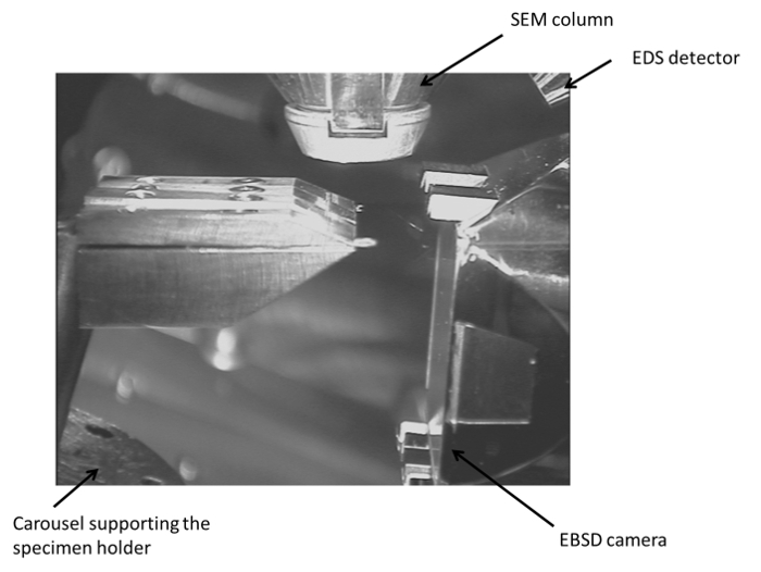
Figure 2. Experimental set-up. The specimen is at a horizontal position after the rotation of the stage. This limits the interference of the stage and carousel with the signal that will be collected on the phosphorus screen of the EBSD camera. Please click here to view a larger version of this figure.

3. EBSD Software Parameters for Data Acquisition

NOTE: The data acquisition parameters are different for specific commercially-available EBSD systems. This section is written as generally as possible, but some of the names and values of the parameters given here are only appropriate if one uses the EBSD software mentioned in the Materials List, and users of different systems will need to adjust these parameters according to their own system. Most of these steps are exactly the same as for a normal EBSD experiment.

1. Make sure that the specimen geometry in the EBSD software reflects the fact that the specimen is in horizontal position. Ensure that the total tilt value is 0°. If not, add a -20° pre-tilt value in the specimen geometry tab.
2. Select the phase(s) (which element or compound) to be analyzed as for a normal EBSD experiment in the phase tab.
3. Capture an image using the EBSD software in the scan image tab by clicking on start.
   NOTE: Forescatter detectors mounted below the EBSD detector phosphor screen can be used to produce a dark field image, assisting in the identification of thin regions and sites of interest.
4. Adjust the settings of the EBSD camera for an optimal data acquisition by optimizing the gain and exposure values until the image is bright but not oversaturated, as for a normal EBSD experiment, in the optimization pattern tab.
   NOTE: This step is dependent on the specimen and its quality (thickness and surface finish).
5. Collect a background in the optimization pattern tab by clicking on collect. Ensure that enough grains are present for the background collection by adjusting the magnification, although it is important to scan across a region with similar thickness to the area to be analyzed.
6. Check the quality of the patterns once the background has been subtracted by ensuring that static background and auto background options have been checked.
   1. Although they will look distorted due to the special geometry of the set-up, ensure that diffraction bands are clearly visible (see Figure 3). Integrate successive frames in the EBSD camera to improve the signal to noise ratio in the image since the luminous intensity of the diffraction pattern on the phosphor screen is low.
   2. If the quality of the patterns is not good enough, change the camera setting (adjust gain and exposure) or change the aperture size of the SEM (use a larger aperture if possible). It might also be due to the specimen being too thick in which case thinning the specimen is the only solution (depending on the specimen this can be done by using a FIB or ion thinning).

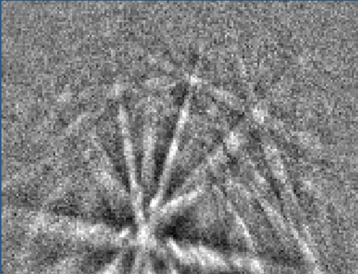
Figure 3. Kikuchi diffraction pattern obtained by TKD. The pattern appears distorted in comparison to a pattern obtained by traditional EBSD and the pattern center has been shifted downwards. Please click here to view a larger version of this figure.

7. Optimize the solver for pattern recognition and to improve the indexing rate by going to the optimize solver tab.
   NOTE: In the software used here, two options are available for better TKD pattern indexing: Optimized TKD or Refined Accuracy. It is recommended to use the Optimized TKD option when the diffraction patterns are highly binned; for higher resolution patterns (e.g. 336 x 256 pixels or higher), the refined accuracy mode works best.
8. If a high resolution analysis is required (a step size of 5 nm or smaller) leave the specimen in the present setting for 30 to 60 min to improve vacuum and thermal beam stability. Do not leave the beam though on the region of interest.
9. Before starting the data acquisition, adjust again the focus and correct the astigmatism of the SEM by repeating step 2.11.
10. Set the parameters (step size and size of the map) for map acquisition in the Acquire Map Data tab.
    NOTE: The step size can be as low as 2 nm if required and if the specimen is of high quality.
11. Start the map acquisition by pressing the start button in the Acquire Map Data tab.
    NOTE: The data analysis will be carried out exactly the same way as for a normal EBSD scan, no adjustments are necessary. Different types of map can be obtained from the data. Euler, band contrast, inverse pole figure, phase maps can all be obtained from the data collected. Pole figures can also be drawn from these data.

Results

The data presented here have been collected using the SEM, EBSD system and software mentioned in the Materials List. Depending on the features of interest, scans were run with different step sizes and the specific step size is indicated for each specimen shown in this work.

The two first examples of TKD application presented here are related to grain refinement of metallic alloys in order to increase their mechanical properties. Stainless steels and Cobalt-Chromium-Molybdenum alloys are commonly used for biomedical applications due to their high corrosion resistance, good mechanical properties under static loading and biocompatibility^23,24. However, both these materials have drawbacks: stainless steels have low hardness and wear resistance while Co-Cr-Mo alloys can fail due to tribocorrosion phenomena. One way to address these materials' short-comings is to change their surface properties by microstructure refinement. Stainless steel and Co-Cr-Mo alloy specimens were subjected to Surface Mechanical Attrition Treatment (SMAT), which is a surface treatment that generates, by severe plastic deformation, a nanocrystalline surface layer that enhances the surface mechanical, tribological, and corrosion properties of bulk materials without changing their chemical composition²⁵. Using TKD, the microstructure below the treated surface was analyzed for the different materials to link the change of microstructure to the improved properties.

Microstructure characterization using TKD has proven that subjecting a stainless steel specimen to SMAT created a region, 1 µm thick below the treated surface, where a mixture of equiaxed nano-grains and slightly elongated nano-grains were present²³. Figure 4 presents one of the TKD scans that were run on a treated sample. The TKD specimen was prepared by using a FIB as the area of interest was just at the surface of the sample. Figure 4 shows that, in the first region below the treated surface, the equiaxed grains are smaller than 100 nm in diameter while the elongated grains present thicknesses of 100 to 200 nm for lengths that can reach 500 nm. Below this first region, a UFG region of elongated sub-micron sized grains can also be seen on the figure. This was the first time that the nano-grain region was properly characterized in a specimen subjected to SMAT. For comparison, another specimen of stainless steel subjected to SMAT was analyzed using traditional EBSD and the results of one of the scans are shown in Figure 5. Both the band contrast and IPF maps show the presence of an UFG region at the surface. However, although a step size of 15 nm was used to run the scan, the grains in that region could not be successfully indexed due to the larger interaction volume that is analyzed at each location during the scan. This shows the limit of the EBSD technique for characterizing UFG and nanocrystalline materials.

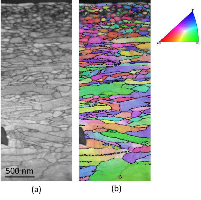
Figure 4. TKD data collected from a stainless steel specimen after SMAT. The data was collected using a step size of 5 nm on a 100 to 120 nm thick specimen. (a) Band contrast map giving an indication of the quality of the collected pattern (the lighter the grey the better the pattern); (b) Inverse Pole Figure (IPF) map showing the different crystallographic orientations of the grains according to the color scheme represented on the right of the map. The surface treated is on the top of the maps. Please click here to view a larger version of this figure.

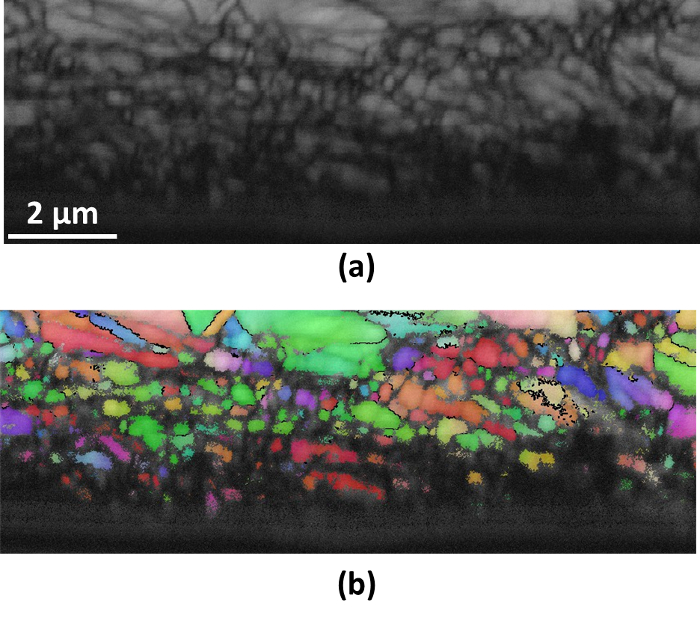
Figure 5. EBSD data collected from a stainless steel specimen after SMAT. The data was collected using a step of 15 nm. (a) Band contract map; (b) IPF map. Please click here to view a larger version of this figure.

Figure 6 illustrates the results of the TKD characterization of a Co-Cr-Mo alloy sample subjected to SMAT. The TKD specimen was prepared using a FIB and the analyzed area was located roughly 10 µm below the treated surface. The results show that a refinement of the microstructure took place via phase transformation²⁴. Initially, the material possessed a single face-centered cubic (fcc) phase and had an average grain size of 10 µm. Figure 6 shows that two phases in this deformed region are present: hexagonal close-packed (hcp) laths are seen inside the fcc grains. The thickness of these laths can be as small as 10 to 20 nm. This refinement of the microstructure explains the three-fold increase in the measured hardness of the material just below the treated surface²⁴.

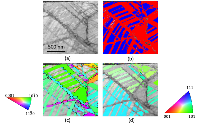
Figure 6. TKD data collected from a Cobalt-Chromium-Molybdenum alloy specimen after SMAT. The data was collected using a step size of 5 nm on a 100 to 120 nm thick specimen. (a) Band contrast map; (b) phase map showing the distribution of the two phases present in the alloy after plastic deformation, the red color represents the hcp phase, while the blue color shows the fcc phase; (c) IPF map showing the different crystallographic orientations of the grains of the hcp phase according to the color scheme represented on the left of the map; (d) IPF map showing the different crystallographic orientations of the grains of the fcc phase according to the color scheme represented on the right of the map. Please click here to view a larger version of this figure.

The last two examples presented here are related to the field of geology. Sub-micron structures can be present in minerals due to the severe plastic deformation they are subjected to within the Earth's mantle or during earthquakes, for example. These materials can present high dislocation densities that make their characterization using traditional EBSD impossible. Detailed study of their microstructure is however paramount to determine the background of these minerals and to understand the different chemical and physical processes to which they have been subjected. For example, it is possible to follow the carbon cycle in the deep Earth by studying diamonds and their inclusions. Figure 7 illustrates one of these studies, where Jacob et al. investigated the microstructure and composition of FeNi-sulfide inclusions in a polycrystalline diamond aggregate that displays a nanogranular magnetite reaction corona²⁶. The TKD analysis revealed the distribution of the different phases present in the specimen (Figure 7b), and showed the nano-structures of the magnetite (Figure 7a). By coupling TKD with EDS, the distribution of the different elements (here showing only Fe and Cu distributions in Figures 7c and d) within the different phases was determined. The study proved that the diamond formed and nucleated by a redox reaction involving the diamond-forming fluid and the FeNi sulfide that formed magnetite and diamond²⁶.

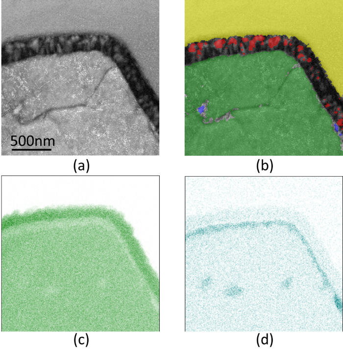
Figure 7. TKD and EDS data collected from FeNi-sulfide inclusions in a polycrystalline diamond aggregate. The data was collected using a step size of 10 nm on an 80 to 100 nm thick specimen. (a) Band contrast map; (b) phase map showing the distribution of the different phases present in specimen, diamond is indicated in yellow, magnetite in red, pyrrhotite in green and chalcopyrite in blue; (c) chemical composition map showing the distribution of Fe in the specimen; (d) chemical composition map showing the distribution of Cu in the specimen. Please click here to view a larger version of this figure.

Many geological samples are subjected to high plastic deformation, although this is not always associated with the Earth's tectonic processes. Impact structures are observed in many meteorite craters on the surface of the Earth, occasionally associated with high enough pressures to transform graphite into diamond²⁷. The structure of these diamonds is highly deformed with very high dislocation densities due to the high energy impact caused by the meteorite. Figure 8 shows an example of an impact diamond characterized using TKD. The large plastic deformation seen by the specimen explains the presence of sub-micron sized grains, a high proportions of twins (see Figure 8b) and gradients of crystallographic orientations within the grains (these gradients are due to high dislocation densities within the grains).

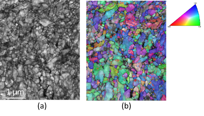
Figure 8. TKD data collected from a meteorite impact diamond. The data was collected using a step size of 10 nm on an 80 to 100 nm thick specimen. (a) Band slope map giving an indication of the quality of the collected pattern (the lighter the grey the better the patter); (b) IPF map showing the different crystallographic orientations of the grains according to the color scheme represented on the right of the map. The red lines represent twin boundaries, with a 60° rotation about <111>. Please click here to view a larger version of this figure.

Discussion

All the data presented in this paper were obtained using a standard, commercial EBSD system. Such a system is available in many laboratories around the world, which means that this technique can readily be applied in these laboratories without having to make any further investment. No modification in the configuration of the SEM and no additional software are necessary to use the EBSD system to collect TKD data. Therefore the transition from traditional EBSD to TKD is very easy. The data acquisition rate for TKD is similar to that of EBSD, which currently reaches up to approximately 1,000 patterns/s¹⁹. This high rate is partially due to the very high level of automation of the technique, including calibration for pattern center position and pattern center change during scanning¹⁹. TKD will benefit from all of these advantages. Additionally, TKD like EBSD, can be coupled easily with EDS to obtain additional chemical information (see Figure 7).

Sample preparation is very important to obtain data in TKD, therefore time should be spent on step 1.2 to insure that the specimen is thin enough to be analyzed. Otherwise there is no point in starting the experiment. Properly setting the parameters of the SEM is paramount in obtaining reliable data. Users should particularly pay attention to steps 2.5 and 2.11 and the values for the parameters given in the protocol might need to be adjusted to specific SEM, EBSD systems and specimens. The parameters to optimize pattern recognition (step 3.7) are also very important to ensure good quality of the data collected. These parameters need to be tested for various patterns in different regions of the area to be scanned to make sure that the complete area of interest can be scanned properly with a high indexing rate.

The different examples presented in this paper attest to the high resolution capability of the technique in comparison with traditional EBSD. Despite the progress made with the hardware and software of the SEM and EBSD systems, the resolution of the EBSD technique cannot reach values below 20 nm for high density materials¹⁷, which means that characterizing features smaller than 50 nm in these materials will be impossible. Working with less dense materials will increase the size of the smallest resolvable feature to the 100 nm mark. Figure 6b shows that it is possible to use TKD to characterize features, such as the hcp laths present in the deformed Co-Cr-Mo alloys, which are as small as 10 to 20 nm, as the spatial resolution of the technique can be as low as 2 nm¹⁷.

Geological materials are usually non-conductive or semi-conductive, which often poses some difficulties when they need to be characterized using traditional EBSD. This problem does not present itself while using TKD. The interaction volume during the analysis is so small given the thin geometry of the specimen that there is no problem of conductivity. This small interaction volume is also an advantage while working with highly deformed materials as normally high dislocation densities makes it impossible to obtain patterns that can be indexed using traditional EBSD. As can be seen in Figure 8, the highly deformed diamond could be characterized using TKD despite the high dislocation densities present in its grains.

One limitation of the technique concerns sample preparation. It is harder to obtain a good specimen for TKD than it is for EBSD. The sample preparation techniques are the same as for TEM sample preparation, which means they are difficult and time-consuming. Finding the correct area to analyze is also a challenge that can be addressed using site specific techniques such as by using a FIB if it is adequate for the type of specimen to be studied. The spatial resolution is improved quite significantly with TKD in comparison with EBSD but is still not as good as what can be attained using TEM^17,19.

This paper has demonstrated that TKD is a valuable technique to characterize nanocrystalline and UFG materials from diverse origins. Its ease of application, speed, resolution and flexibility in term of conductivity outweigh the difficulty in sample preparation. The future of the technique resides in in situ characterization. By using an in situ mechanical testing rig while carrying out TKD analysis, it will be possible to observe how these nano- and ultra-fine microstructures change under external loading. This will increase our knowledge on the deformation mechanisms of nanocrystalline and UFG materials.

Materials

List of materials used in this article

Name	Company	Catalog Number	Comments
Scanning electron microscope	Zeiss		Preferably equipped with a  field emission source in order to maximize spatial resolution. The one used here is a Zeiss Ultra plus field emission-SEM
Electron backscatter diffraction detector	Oxford instruments		Different system are available on the market. The one is in this work is a Nordlys-nano EBSD detector from Oxford instruments. Forescatter detectors are mounted belown the detector phospor screen which is an option.
Electron backscatter diffraction software for data acquisition and analysis	Oxford instruments		The protocal is described here for the usage of the AZtecHKL EBSD software but other software can be used as well
EDS detector	Oxford instruments		This is optional. The one used here is a X-Max 20 mm2 silicon drift EDS detector from Oxford instruments
sample holder for TKD	ANY		As long as it can handle thin specimen and can be placed in the correct orientation within the microscope. Different companies sell specific sample holders for TKD analysis if required by the user.
Plasma cleaner	Evactron		This is optional. The one used here is Evactron Model 25 RF Plasma Decontaminator for FIB/SEM and Vacuum Chambers

References

- Wang, Y. M., Chen, M. W., Zhou, F. H., Ma, E. High tensile ductility in a nanostructured metal. Nature. 419, 912-915 (2002).
- Liddicoat, P. V., et al. Nanostructural hierarchy increases the strength of aluminium alloys. Nat. Commun. 1 (63), 1-7 (2010).
- Mukai, T., Yamanoi, M., Watanabe, H., Higashi, K. Ductility enhancement in AZ31 magnesium alloy by controlling its grain structure. Scr. Mater. 45 (1), 89-94 (2001).
- Liao, X. Z., Zhao, Y. H., Zhu, Y. T., Valiev, R. Z., Gunderov, D. V. Grain size effect on the deformation mechanisms of nanostructured copper processed by high-pressure torsion. J. Appl. Phys. 96, 636-640 (2004).
- Fang, Z. Z., Wang, H. Densification and grain growth during sintering of nanosized particles. Int. Mater. Rev. 53 (6), 326-352 (2008).
- Handtrack, D., Despang, F., Sauer, C., Kieback, B., Reinfried, N., Grin, Y. Fabrication of ultra-fine grained and dispersion-strengthened titanium materials by spark plasma sintering. Mater. Sci. Eng., A. 437 (2), 423-429 (2006).
- Bestmann, M., Pennacchioni, G., Frank, G., Göken, M., de Wall, H. Pseudotachylyte in muscovite-bearing quartzite: Coseismic friction-induced melting and plastic deformation of quartz. J. Struct. Geol. 33 (2), 169-186 (2011).
- Trepmann, C. Shock effects in quartz: Compression versus shear deformation - An example from the Rochechouart impact structure, France. Earth Planet. Sci. Lett. 267 (1-2), 322-332 (2008).
- Pearce, M. A., Gazley, M. F., Fisher, L. A., Saunders, M., Hough, R. M., Kong, C. The Nanostructure of Australia's Gold Deposits. Proceeding of AMAS XIII - 13th Biennial Australian Microbeam Analysis Symposium, Hobart, Australia, , (2015).
- Mukai, H., Saruwatari, K., Nagasawa, H., Kogure, T. Aragonite twinning in gastropod nacre. J. Cryst. Growth. 312 (20), 3014-3019 (2010).
- Daly, L., Bland, P. A., Trimby, P. W., Moody, S., Yang, L., Ringer, S. P. Transmission Kikuchi diffraction applied to primitive grains in meteorites. Lunar and Planetary Science Conference. 46, 1752(2015).
- Rauch, E. F., Véron, M. Automated crystal orientation and phase mapping in TEM. Mater. Charact. 98, 1-9 (2014).
- Humphreys, F. J., Brough, I. High resolution electron backscatter diffraction with a field emission gun scanning electron microscope. J. Microsc. 195, 6-9 (1999).
- Zhilyaev, A. P., Kim, B. K., Nurislamova, G. V., Baro, M. D., Szpunar, J. A., Langdon, T. G. Orientation imaging microscopy of ultrafine-grained nickel. Scr. Mater. 46 (8), 575-580 (2002).
- Apps, P. J., Bowen, J. R., Prangnell, P. B. The effect of coarse second-phase particles on the rate of grain refinement during severe deformation processing. Acta Mater. 51 (10), 2811-2822 (2003).
- Dogan, E., Vaughan, M. W., Wang, S. J., Karaman, I., Proust, G. Role of starting texture and deformation modes on low-temperature shear formability and shear localization of Mg-3Al-1Zn alloy. Acta Mater. 89, 408-422 (2015).
- Trimby, P. W. Orientation mapping of nanostructured materials using transmission Kikuchi diffraction in the scanning electron microscope. Ultramicroscopy. 120, 16-24 (2012).
- Schwarzer, R. A. Advances in crystal orientation mapping with the SEM and TEM. Ultramicroscopy. 67 (1-4), 19-24 (1997).
- Zaefferer, S. A critical review of orientation microscopy in SEM and TEM. Cryst. Res. Technol. 46 (6), 607-628 (2011).
- Keller, R. R., Geiss, R. H. Transmission EBSD from 10 nm domains in a scanning electron microscope. J. Microsc. 245 (3), 245-251 (2012).
- Trimby, P., et al. Characterizing deformed ultrafine-grained and nanocrystalline materials using transmission Kikuchi diffraction in a scanning electron microscope. Acta Mater. 62, 69-80 (2014).
- Ayache, J., Beaunier, L., Boumendil, J., Ehret, G., Laub, D. Sample Preparation Handbook for Transmission Electron Microscopy: Methodology. , Springer. Berlin/Heidelberg. (2010).
- Proust, G., Retraint, D., Chemkhi, M., Roos, A., Demangel, C. Electron Backscatter Diffraction and Transmission Kikuchi Diffraction Analysis of an Austenitic Stainless Steel Subjected to Surface Mechanical Attrition Treatment and Plasma Nitriding. Microsc. Microanal. 21 (4), 919-926 (2015).
- Proust, G., Retraint, D., Raoult, A. G., Demangel, C., Tchana, D., Benhayoune, H. Microstructural Characterization of a Cobalt-Chromium-Molybdenum Alloy Subjected to Surface Mechanical Attrition Treatment. Proceedings of PLASTICITY '16: The Twenty Second International Symposium on Plasticity and its Current Applications, , 46-48 (2016).
- Lu, K., Lu, J. Nanostructured surface layer on metallic materials induced by surface mechanical attrition treatment. Mater. Sci. Eng., A. 375-377, 38-45 (2004).
- Jacob, D. E., Piazolo, S., Schreiber, A., Trimby, P. Redox-freezing and nucleation of diamond via magnetite formation in the Earth's mantle. Nat. Commun. 7, Article number: 11891(2016).
- Kvasnytsya, V., Wirth, R., Piazolo, S., Jacob, D. E., Trimby, P. Surface morphology and structural types of natural impact apographitic diamonds. J. Superhard Mater. 38 (2), 71-84 (2016).
Reprints and Permissions