Surface Mapping of Earth-like Exoplanets using Single Point Light Curves

Summary

The protocol extracts information from light curves of exoplanets and constructs their surface maps. It uses light curves of Earth, which serves as a proxy exoplanet, to demonstrate the approach.

Abstract

Spatially resolving exoplanet features from single-point observations is essential for evaluating the potential habitability of exoplanets. The ultimate goal of this protocol is to determine whether these planetary worlds harbor geological features and/or climate systems. We present a method of extracting information from multi-wavelength single-point light curves and retrieving surface maps. It uses singular value decomposition (SVD) to separate sources that contribute to light curve variations and infer the existence of partially cloudy climate systems. Through analysis of the time series obtained from SVD, physical attributions of principal components (PCs) could be inferred without assumptions of any spectral properties. Combining with viewing geometry, it is feasible to reconstruct surface maps if one of the PCs are found to contain surface information. Degeneracy originated from convolution of the pixel geometry and spectrum information determines the quality of reconstructed surface maps, which requires the introduction of regularization. For the purpose of demonstrating the protocol, multi-wavelength light curves of Earth, which serves as a proxy exoplanet, are analyzed. Comparison between the results and the ground truth is presented to show the performance and limitation of the protocol. This work provides a benchmark for future generalization of exoplanet applications.

Introduction

Identifying habitable worlds is one of the ultimate goals in astrobiology¹. Since the first detection², more than 4000 exoplanets have been confirmed to date³ with a number of Earth analogs (e.g., TRAPPIST-1e)⁴. These planets have orbital and planetary properties similar to those of Earth, and therefore are potentially habitable. Evaluating their habitability from limited observations is essential in this context. Based on the knowledge of life on Earth, geological and climate systems are critical to habitability, which can therefore serve as biosignatures. In principle, features of these systems could be observed from a distance even when a planet could not be spatially resolved better than one single point. In this case, identifying geological features and climate systems from single-point light curves is essential when assessing the habitability of exoplanets. Surface mapping of these exoplanets becomes urgent.

Despite the convolution between viewing geometry and spectral features, information of an exoplanet’s surface is contained in its time-resolved single-point light curves, which can be obtained from a distance, and derived with sufficient observations. However, two-dimensional (2D) surface mapping of potentially habitable Earth-like exoplanets is challenging due to the influence of clouds. Methods of retrieving 2D maps have been developed and tested using simulated light curves and known spectra^5,6,7,8, but they have not been applied to real observations. Moreover, in the analyses of exoplanet observations now and in the near future, assumptions of characteristic spectra may be controversial when the planetary surface compositions are not well-constrained.

In this paper, we demonstrate a surface mapping technique for Earth-like exoplanets. We use SVD to evaluate and separate information from different sources that is contained in multi-wavelength light curves without assumptions of any specific spectra. Combined with viewing geometry, we present the reconstruction of surface maps using timely resolved but spatially convoluted surface information. For the purpose of demonstrating this method, two-year multi-wavelength single-point observations of Earth obtained by the Deep Space Climate Observatory/Earth Polychromatic Imaging Camera (DSCOVR/EPIC; www.nesdis.noaa.gov/DSCOVR/spacecraft.html) are analyzed. We use Earth as a proxy exoplanet to assess this method because currently available observations of exoplanets are not sufficient. We attach the code with the paper as an example. It is developed under python 3.7 with anaconda and healpy packages, but the mathematics of the protocol can also be done in other programming environments (e.g., IDL or MATLAB).

Protocol

1. Programming setup

1. Set up the programming environment for the attached code. A computer with Linux operating system is required, as the healpy package is not available on Windows. The code is not computationally expensive, so a normal personal computer can handle the protocol.
2. Follow the instruction (https://docs.anaconda.com/anaconda/install/linux/) to install Anaconda with Python 3.7 onto the system, then use the following commands in terminal to set up the programming environment:
   $ conda create --name myenv python=3.7
   $ conda activate myenv
   $ conda install anaconda
   $ conda install healpy
   NOTE: These steps may take tens of minutes depending on the hardware and Internet speed. The environment name ‘myenv’ in the first two command lines can be changed to any other string.

2. Obtaining multi-wavelength light curves and viewing geometry from observations

1. In the viewing geometry, include the longitude and latitude of the sub-stellar and the sub-observer points for each corresponding time frame.
   To use the following attached code, ensure that these two files have the same format as LightCurve.csv and Geometry.csv.
2. Run PlotTimeSeries.py to visualize the data and check their qualities. Two figures LightCurve.png and Geometry.png will be created (Supplemental Figure 1-2). Parameters in this and following plotting codes may need to be adjusted if applied to different observations.
   $ python PlotTimeSeries.py LightCurve
   $ python PlotTimeSeries.py Geometry

3. Extract surface information from light curves

1. Center time-resolved multi-wavelength albedo light curves of an exoplanet and normalize them by corresponding standard deviation at each wavelength. This results in the equal importance of each channel.
   
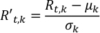
   where R’_t,k and R_t,k are the scaled and observed albedo at the t-th time step and the k-th wavelength, respectively; μ_k and σ_k are the mean and standard deviation of the albedo time series at the k-th wavelength.
   1. Run Normalize.py to normalize the light curves, R_t,k. The output is saved in NormalizedLightCurve.csv.
      $ python Normalize.py
2. Run PlotTimeSeries.py to visualize the normalized light curves. A figure NormalizedLightCurve.png will be created (Supplemental Figure 3).
   $ python PlotTimeSeries.py NormalizedLightCurve
3. Apply SVD on the scaled albedo light curves to find dominant PCs and their corresponding time series.
   
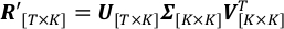
   On the left hand side, T and K are the total number of time steps and observation wavelengths; R’ is the matrix of scaled albedo observations, whose (t,k)-th element is R’_t,k. On the right hand side, columns of V are PCs, orthonormal vectors that define the space SVD projects to; Σ is a diagonal matrix, whose (k,k)-th element is the standard deviation of scaled light curves along the k-th axis defined by the k-th column of V; columns of U are the corresponding time series of each PC in V.
   1. Run SingularValueDecomposition.py to decompose R’. The resulting U, Σ, V^T are saved in the output files U.csv, SingularValue.csv and V_T.csv, respectively.
      $ python SingularValueDecomposition.py
4. Use PlotTimeSeries.py and PlotSVD.py to visualize the SVD result. Three figures U.png, Sigma.png and V_T.png will be created (Supplemental Figure 4-6).
   $ python PlotTimeSeries.py U
   $ python PlotSVD.py
5. Analyze contributions and corresponding time series of PCs to determine the one that contains surface information.
   1. Compare the singular values at the diagonal of Σ. An Earth-like partially cloudy exoplanet is expected to have two comparable dominant singular values.
      NOTE: Σ may contain less or more than two dominant singular values, which is discussed below.
   2. Compare the time series patterns of the two dominant PCs. The PC that contains surface information tends to have more regular shape than the other. Due to the longitudinal asymmetry and the reappearance of surface with small changes in two consecutive days, the corresponding time series tends to have approximately constant daily variation.
   3. Compute the periodicities of the two dominant PCs using Lomb-Scargle periodogram^9,10 to confirm the selection of PC. The PC that contains surface information tends to have higher peak corresponding to rotation period in the power density spectrum.
   4. Run Periodogram.py to obtain the power spectra of the time series of each PC. The power spectra are saved in Periodogram.csv.
      $ python Periodogram.py
   5. Run PlotPeriodogram.py to visualize these periodograms and confirm the selection of PC. A figure Periodogram.png will be created (Supplemental Figure 7). The current plotting code adds in dashed lines representing annual, semi-annual, diurnal and half-daily cycles for reference, which may need to be changed when applied to other observations.
      $ python PlotPeriodogram.py
   6. Select the PC, v_j, that contains surface information and its time series, u_j.
      
      
      where V[:,j] and U[:,j] are the j-th columns of V and U, respectively; j is the index of PC inferred at step 3.3 that contains surface information.

4. Construct planetary surface map

1. Use the Hierarchical Equal Area iso-Latitude Pixelization (HEALPix)¹¹ method to pixelate the retrieving map. It divides spherical surface of a planet into pixels with the same area and uniform distribution. Denote the unknown value of the p-th pixel as x_p.
   1. Run HEALPixRandom.py to visualize the pixelization method. A figure HEALPixRandom.png will be created (Supplemental Figure 8). The parameter N_side at line 17 can be changed for different resolutions. This step may take a few seconds to minutes depending on the resolution.
      $ python HEALPixRandom.py
2. Compute the weight of the p-th pixel in observations at the t-th time step, w_t,p, using viewing geometry.
   
   where α_t,p, β_t,p are the solar and the spacecraft zenith angles at the p-th pixel at the t-th time step; c_t is a normalization term of the t-th observation so that sum of the total weight at each time step is unity.
   NOTE: Geometry is assumed to be known at this step, or can be derived from other analysis, which is discussed below.
   1. Run ComputeWeight.py to compute w_t,p. Change the value of N_side at line 23 for other resolutions of the retrieved map. The output is saved as W.npz due to its size.
      $ python ComputeWeight.py
3. Use PlotWeight.py to visualize these weights. A number of figures, one at each time step, will be created in a folder Weight. Merging them results in Supplemental Video 1, which shows how the weight of each pixel changes with time. This step may take hours to finish due to the large number of visualizations.
   $ python PlotWeight.py
4. Combine geometry and observations to reach a linear regression problem.
   
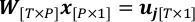
   where P is the total number of retrieving pixels; W is the weight matrix with w_t,p as the (t,p)-th element; x consists of x_p as the p-th element, which is the quantity to be solved in this problem.
   Solve the linear regression problem with a regularization of L-2 norm.
   
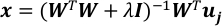
   where I is the identity matrix and λ is the regularization parameter.
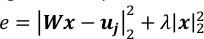
   NOTE: 10^-3 is a good value for λ when T~10⁴ and P~3*10³. They should be adjusted by comparing the values of the two terms in the regularized square error, e, as shown below.
   
   1. Run LinearRegression.py to solve this linear regression problem. The result of x is saved in the file PixelValue.csv. Change the value of λ at line 16 for different strengths of regularization.
      $ python LinearRegression.py
5. Convert x to a 2D surface map according to the mapping rule of HEALPix.
   1. Run PlotMap.py to construct the retrieved maps using different regularization parameters. Three figures Map_-2.png, Map_-3.png and Map_-4.png will be created with the current setting (Supplemental Figure 9). The relationship between the pixel indices and their locations on map is described in the HEALPix document¹¹. This step takes tens of seconds.
      $ python PolotMap.py

5. Estimate uncertainty of the retrieved map

1. Rewrite the linear regression problem at step 4.3 with the “true value” of x as z and the observation noise, ε.
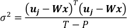
   1. Assume ε to follow a Gaussian Distribution N (0, σ²I_[T*T]) and estimate its covariance. T-P is the degree of freedom of u_j from observation when the retrieved map is fixed.
      
   2. Combine equations in step 4.4 and 5.1. It results in a Gaussian vector of x.
      
   3. Compute the expectation and the covariance matrix of x.
      
   4. Obtain the uncertainty of each element in x as the square root of the corresponding element on the diagonal of Cov[x].
      
      where e_p is the uncertainty of x_p; Diag[Cov[x]]_p is p-th element on the diagonal of Cov[x].
   5. Run Covariance.py to compute the covariance matrix of x. The result is saved in Covariance.npz due to its size. This step takes tens of seconds to minutes depending on the size of W.
      $ python Covariance.py
2. Convert e_p to the retrieved 2D map according to the mapping rule of HEALPix.
   1. Run PlotCovariance.py to visualize Cov[x] and map the uncertainty e_p to the retrieved map. Two figures Covariance.png and Uncertainty.png will be created (Supplemental Figure 10-11).
      $ python PlotCovariance.py

Representative Results

We use multi-wavelength single-point light curves of Earth to demonstrate the protocol, and compare the results with the ground truth to evaluate the quality of surface mapping. Observation used here is obtained by DSCOVR/EPIC, which is a satellite located near the first Lagrangian point (L1) between Earth and Sun taking images at ten wavelengths of the sunlit face of Earth. Two years (2016 and 2017) of observations are used for this demonstration, which are the same as those in Jiang et al. (2018)¹² and Fan et al. (2019)¹³, where more details about the observations are presented. A sample observation at 9:27 UTC, 2017 February 8 is shown in Figure 1. Images of Earth are integrated to single points to simulate light curve observations obtained by Aliens, distant observers, who could not spatially resolve Earth better than one pixel. Therefore, multi-wavelength single-point exoplanet light curves with ~10,000 time steps are generated, which are the input data of this protocol.

Following step 3, we find two dominant PCs in the multi-wavelength light curves, and the second PC (PC2) contains surface information. Derived as step 3.5, time series of PC2 shows more regular morphology with an approximately constant daily variation, and its power spectrum shows stronger diurnal cycle than the first PC (PC1, Figure 2). Therefore, a surface map of this proxy exoplanet is constructed following step 4 (Figure 3a), which consists of the value of PC2 at each pixel. Compared with the ground truth of Earth (Figure 3b), the reconstructed map recovers all major continents, despite some disagreements in the southern hemisphere where clouds partially prevent surface information from being observed. Uncertainty of each pixel value obtained according to step 5 (Figure 3c) is on the order of 10% of that in the retrieved map, suggesting a good quality of the surface mapping and a positive result.

Figure 1: Reflectance images of Earth’s sunlit hemisphere.
The observations are taken by DSCOVR/EPIC at ten wavelengths and at 9:27 UTC, 2017 February 8. Please click here to view a larger version of this figure.

Figure 2: Time series and power spectra of the two dominant PCs.
(a) Time series of PC1. Daily maximum and minimum are denoted by black lines. (b) Power spectrum of PC1’s time series. Annual, semi-annual, diurnal and half-daily cycles are denoted as black dashed line. (c) and (d) are identical to (a) and (b), but correspond to PC2. This figure is taken from Fan et al. (2019)¹³. Please click here to view a larger version of this figure.

Figure 3: Reconstruction of Earth’s surface.
(a) Surface map of Earth, which serves as a proxy exoplanet, reconstructed from multi-wavelength light curves. Colors in the map are the values of PC2 at each pixel. The contour of median value is denoted as the black line. (b) Ground truth of Earth’s surface map. (c) Uncertainty of the reconstructed map shown in (a). This figure is modified from Fan et al. (2019)¹³. Please click here to view a larger version of this figure.

Figure 4: Result of finding the optimal regularization parameter.
The optimal value of the regularization parameter λ is 10^-3.153 (dashed line) when χ² of the reconstruction (solid line) reaches its minimum. Please click here to view a larger version of this figure.

Figure 5: Sensitivity test of observation noise.
(a) Correlation coefficient between PC2 and land fraction in the field of view (solid line) derived from observations with different signal to noise ratios (S/Ns). The original correlation from light curves without noise is shown as the dashed line. (b) The importance of each PC on the land fraction derived with different observation S/Ns. The importance is computed using Gradient Boosted Regression Trees (GBRT) models as described in Fan et al. (2019)¹³. Please click here to view a larger version of this figure.

Supplemental Figure 1: Time series of reflectance of Earth at ten wavelengths. Please click here to download this figure.

Supplemental Figure 2: (a) Time series of latitude of the sub-observer point. (b) Same as (a), but for longitude. (c) and (d) are identical to (a) and (b), but correspond to the sub-stellar point. Please click here to download this figure.

Supplemental Figure 3: Time series of normalized reflectance of Earth at ten wavelengths. Please click here to download this figure.

Supplemental Figure 4: Time series of the ten PCs, columns of U. Please click here to download this figure.

Supplemental Figure 5: Singular values corresponding to each PC, diagonal elements of Σ. Please click here to download this figure.

Supplemental Figure 6: Normalized reflectance spectra of ten PCs, columns of V. Please click here to download this figure.

Supplemental Figure 7: Power density spectra of time series of ten PCs. Please click here to download this figure.

Supplemental Figure 8: Pixelization of retrieving map, filled with random pixel values. Please click here to download this figure.

Supplemental Figure 9: Reconstructed map of Earth using different regularization parameters of (a) 10^-2, (b) 10^-3, and (c) 10^-4. Please click here to download this figure.

Supplemental Figure 10: Covariance matrix of x. Please click here to download this figure.

Supplemental Figure 11: Square root of the diagonal elements of the covariance matrix of x, mapped onto the retrieved surface map. Please click here to download this figure.

Video S1: Pixel weights for observations at each time frame in 2016 and 2017.

Supplemental Files.  Please click here to download these files.

Discussion

One critical requirement of the protocol is the feasibility of extracting surface information from light curves, which depends on the cloud coverage. In step 3.5.1, the relative values of the PCs may be different among exoplanets. In the case of Earth, the first two PCs dominate the light curve variations, and correspond to surface-independent clouds and surface (Fan et al. 2019)¹³. They have comparable singular values so that the surface information can be separated following steps 3.5.2 and 3.5.3. For a future observation of exoplanet, in extreme cases of either an entirely cloudy or a cloud-free exoplanet, only one dominant PC would appear in the SVD at step 3.3. Spectral analysis is necessary in this case to interpret the meaning of this PC, as compositions of clouds and surface are different. If the dominant PC corresponds to the surface, step 4 and 5 could still be followed; if it corresponds to clouds, a conclusion can be drawn that surface information is blocked by clouds and therefore cannot be extracted using light curves at given wavelengths. In this case, surface mapping is not feasible. A third or even fourth comparable dominant PC may also exist, which can correspond to another layer of clouds or large-scale hydrological processes, and would not invalidate the following steps of the method as long as the surface information is extracted.

Degeneracy resulting from the convolution of geometry and spectrum is the dominant factor that constrains the quality of the retrieved map, as discussed in Cowan & Strait (2013)¹⁴ and Fujii et al. (2017)¹⁵. As the time series of dominant PCs cover only a small portion of the PC plane, there is always a trade-off between spatial and spectral variations. In other words, the retrieved map (Figure 2a) could not be much improved even with an infinite number of time steps and perfect observations, as long as using light curves at the same wavelengths. We introduce the regularization to partially relieve the degeneracy. The optimal value of the regularization term λ in step 4.4 is determined using observations synthesized by the ground truth, where the observed u_j is replaced by weighted and scaled land fractions in the field of view (FOV). To generate the synthetic observation, we use the equation at step 4.3 and replace x with the ground truth land fractions of each pixel, y. y is scaled to the same range with x using the strong linear correlation between PC2 of observation, u₂, and the averaged FOV land fraction¹³. Due to the degeneracy, y cannot be perfectly recovered from the linear regression in step 4.4, so we determine the optimal value of λ by finding the minimum of χ², squared residual scaled by the variance of each pixel. The latter is estimated by the absolute value of each pixel. This is similar to the L-curve criterion in Kawahara & Fujii (2011)¹⁶. In the particular case of this paper where T=9739 and P=3072, the optimal value of λ is 10^-3.153 (Figure 4).

Observation noise, another factor that influences the mapping quality, may corrupt the SVD analysis of light curves in practical. We test the robustness of the protocol by introducing different levels of observation noise to the original light curves. They are assumed to contain all noise sources (e.g. sky background, dark current and readout noise), and follow Gaussian distribution. In the original light curves without noise, PC2 shows strong (r²=0.91) linear correlation with the FOV land fraction¹³, so its time series is used for the surface mapping. With increasing noise level, the correlation between PC2 and surface becomes weaker (Figure 5). The correlation coefficient, r², becomes below 0.5 when the signal to noise ratio (S/N) is less than 10 (Figure 5a), although the importance of PC2 is still dominant (Figure 5b). We suggest a minimum S/N of 30 for confidently applying the protocol in future generalization. It is worth noting that S/N here is the ratio of exoplanet signal to the observation noise, with the signal of parent star being removed.

Viewing geometry is assumed to be known at step 4.2, as precisely deriving viewing geometry from exoplanet observations is beyond the scope of this work. Besides the orbital elements that can be derived from light curve observations, and rotation period from power density spectra (Figure 2b and 2d), there are only two quantities, summer/winter solstice and obliquity, that are required for surface mapping. Summer/winter solstice usually coincide with extremum of time series of the surface corresponding PC, as long as there exists noticeable asymmetry between northern and southern hemispheres. Obliquity of the exoplanet can be inferred from its influence on the amplitude and frequency of light curves^17,18. All these derivations require observations sampling frequency at least higher than that of planetary rotation, which is currently rarely satisfied for exoplanets.

Materials

Name	Company	Catalog Number	Comments
Python 3.7 with anaconda and healpy packages			Other programming environments (e.g., IDL or MATLAB) also work.

References

- Schwieterman, E. W., et al. Exoplanet Biosignatures: A Review of Remotely Detectable Signs of Life. Astrobiology. 18 (6), 663-708 (2018).
- Campbell, B., Walker, G. A. H., Yang, S. A Search for Substellar Companions to Solar-type Stars. The Astrophysical Journal. 331, 902 (1988).
- NASA. NASA Exoplanet Archive (2019) Confirmed Planets Table. , (2019).
- Gillon, M., et al. Seven temperate terrestrial planets around the nearby ultracool dwarf star TRAPPIST-1. Nature. 542 (7642), 456-460 (2017).
- Kawahara, H., Fujii, Y. Global Mapping of Earth-like Exoplanets from Scattered Light Curves. The Astrophysical Journal. 720 (2), 1333 (2010).
- Fujii, Y., Kawahara, H. Mapping Earth Analogs from Photometric Variability: Spin-Orbit Tomography for Planets in Inclined Orbits. The Astrophysical Journal. 755 (2), 101 (2012).
- Cowan, N. B., Fujii, Y. Mapping Exoplanets. Handbook of Exoplanets. , Springer, Cham. (2018).
- Farr, B., Farr, W. M., Cowan, N. B., Haggard, H. M., Robinson, T. exocartographer: A Bayesian Framework for Mapping Exoplanets in Reflected Light. The Astronomical Journal. 156 (4), 146 (2018).
- Lomb, N. R. Least-Squares Frequency Analysis of Unequally Spaced Data. Astrophysics and Space Science. 39 (2), 447 (1976).
- Scargle, J. D. Studies in astronomical time series analysis. II. Statistical aspects of spectral analysis of unevenly spaced data. The Astrophysical Journal. 263, 835 (1982).
- Górski, K. M., et al. HEALPix: A Framework for High-Resolution Discretization and Fast Analysis of Data Distributed on the Sphere. The Astrophysical Journal. 622 (2), 759 (2005).
- Jiang, J. H., et al. Using Deep Space Climate Observatory Measurements to Study the Earth as an Exoplanet. The Astronomical Journal. 156 (1), 26 (2018).
- Fan, S., et al. Earth as an Exoplanet: A Two-dimensional Alien Map. The Astrophysical Journal Letters. 882 (1), 1 (2019).
- Cowan, N. B., Strait, T. E. Determining Reflectance Spectra of Surfaces and Clouds on Exoplanets. The Astrophysical Journal Letters. 765 (1), 17 (2013).
- Fujii, Y., Lustig-Yaeger, J., Cowan, N. B. Rotational Spectral Unmixing of Exoplanets: Degeneracies between Surface Colors and Geography. The Astronomical Journal. 154 (5), 189 (2017).
- Kawahara, H., Fujii, Y. Mapping Clouds and Terrain of Earth-like Planets from Photomertic Variability: Demonstration with Planets in Face-on Orbits. The Astrophysical Journal Letters. 739 (2), 62 (2011).
- Kawahara, H. Frequency Modulation of Directly Imaged Exoplanets: Geometric Effect as a Probe of Planetary Obliquity. The Astrophysical Journal. 822 (2), 112 (2016).
- Schwartz, J. C., Sekowski, C., Haggard, H. M., Pall ́e, E., Cowan, N. B. Inferring planetary obliquity using rotational and orbital photometry. Monthly Notices of the Royal Astronomical Society. 457 (1), 926-938 (2016).