A Simple Stimulatory Device for Evoking Point-like Tactile Stimuli: A Searchlight for LFP to Spike Transitions

Summary

To elucidate the complex transition from Local Field Potentials (LFPs) to spikes a suitable stimulator for light mechanical peripheral stimuli was built. As an application, the spiking activities recorded from somatosensory cortex were analyzed by a multi-objective optimization strategy. The results demonstrated that the proposed stimulator was able to deliver tactile stimuli with millisecond and millimeter precisions.

Abstract

Current neurophysiological research has the aim to develop methodologies to investigate the signal route from neuron to neuron, namely in the transitions from spikes to Local Field Potentials (LFPs) and from LFPs to spikes.

LFPs have a complex dependence on spike activity and their relation is still poorly understood¹. The elucidation of these signal relations would be helpful both for clinical diagnostics (e.g. stimulation paradigms for Deep Brain Stimulation) and for a deeper comprehension of neural coding strategies in normal and pathological conditions (e.g. epilepsy, Parkinson disease, chronic pain). To this aim, one has to solve technical issues related to stimulation devices, stimulation paradigms and computational analyses. Therefore, a custom-made stimulation device was developed in order to deliver stimuli well regulated in space and time that does not incur in mechanical resonance. Subsequently, as an exemplification, a set of reliable LFP-spike relationships was extracted.

The performance of the device was investigated by extracellular recordings, jointly spikes and LFP responses to the applied stimuli, from the rat Primary Somatosensory cortex. Then, by means of a multi-objective optimization strategy, a predictive model for spike occurrence based on LFPs was estimated.

The application of this paradigm shows that the device is adequately suited to deliver high frequency tactile stimulation, outperforming common piezoelectric actuators. As a proof of the efficacy of the device, the following results were presented: 1) the timing and reliability of LFP responses well match the spike responses, 2) LFPs are sensitive to the stimulation history and capture not only the average response but also the trial-to-trial fluctuations in the spike activity and, finally, 3) by using the LFP signal it is possible to estimate a range of predictive models that capture different aspects of the spike activity.

Introduction

In the context of signal processing the impulse response provides a fundamental characterization of the behavior of a dynamical system.

Although the ideal impulse stimulus is practically not achievable, it is possible to obtain a reasonable approximation of it by using an actuator element that generates high frequency displacements. This type of light tactile-vibratory stimulation is known to target both deep skin (e.g. fast responding, fast adapting Pacinian corpuscles)² and superficial receptors (e.g. low-threshold slowly adapting Merkel discoid structures)².

Current stimulation devices, mainly piezoelectric actuators, are charged with a number of drawbacks, not least resonances and small displacements. To overcome these flaws, an alternative implementation of impulse-like stimulation is proposed by using a blunted tip (a cactus smoothed tip in our case) vertically mounted on the membrane center of a mid-range speaker cone. This provides the advantage of larger displacements and broader frequency spectrum.

An effective application of such a device was the study of the relevant neurophysiological problem of the LFPs to spikes dependency. Because of the subtle temporal association between these electrical events a finely regulated device was needed for delivering peripheral stimuli. The stimuli had to be as fast and spatially selective as possible in order to reduce the "background noise" and sharpen the signals of interest. To this purpose, the stimulation device and the stimulus delivery protocol were jointly optimized for the task. In this paper, we describe the technique and present some representative results.

A stimulation protocol based on randomized paired-pulses has been designed and optimized in order to avoid habituation. This protocol offered the advantage of classical paired pulses and reduced the possibility of spurious locking between stimuli and spontaneous periodical bursts of neuronal activity.

By using this randomized paired pulse it was possible to obtain fast and reliable LFP and spike responses and to capture the special feature of these responses related to the dependence of both LFPs and spikes on the stimulation history. Indeed, from the raw LFP responses, a set of three LFP features (the LFP itself, the LFP first derivative and phase of the first derivative) strongly correlating with the average spike response, was also extracted.

Few methods have been proposed to fit models that predict spikes from LFPs^3,4. In general a critical point of the model fitting process, common also to the prediction of spike event from the stimulus signal, is constituted by the appropriate choice of the objective function to maximize/minimize. While a range of objective functions has been proposed (e.g. correlation and coherence)⁵ none of these jointly captures the whole complexity of spike responses. Accordingly, a novel framework based on multi-objective optimization is introduced. We show that by using the proposed devised and this computational framework it is possible to estimate a set of predictive models based on strong LFP to spike relationships.

Protocol

Ethical Statement

To study how sensory stimuli are represented by neuronal activity there is no alternative to the use of animals and the use of an in vivo approach. All the animals have been treated along the Italian and European Laws on animal treatment in Scientific Research (Italian Bioethical Committee, Law Decree on the Treatment of Animals in Research, 27 Jan 1992, No. 116). The National Research Council, where the experiments have been performed, adheres to the International Committee on Laboratory Animal Science (ICLAS) on behalf of the United Nations Educational, Scientific and Cultural Organizations (UNESCO), the Council for International Organizations of Medical Sciences (CIOMS) and the International Union of Biological Sciences (IUBS). As such, no protocol-specific approval was required. The approval of the Ministry of Health is classified as "Biella 1, 3/2011" into the files of the Ethical Committee of the University of Milan.

1. Preparation of the Experimental Animals

1. Select male rats approximately 300-400 g in size.
2. Anesthetize the rats for the experimental preparation.
   1. Inject intraperitoneally a barbiturate solution (pentobarbital, 50 mg/kg for induction, 10 mg/kg for maintenance).
   2. Check the anesthesia level by low threshold and high threshold mechanical stimuli over a paw ensuring that no retraction reflex occurs.
   3. Prepare the cranial skin by shaving the cranial vault accurately and then make an incision to expose the cranial surface.
   4. Cannulate the trachea, by a tracheal cannula (inner diameter of 2 mm and outer diameter of 2.5 mm) fixing it by surgical ligation around the trachea itself.
   5. Laterally to the tracheal segment expose the jugular vein and cannulate it inserting a cannula (PE10) connected to a syringe fixing it by surgical ligation around the vessel.
3. Mount the rat onto a stereotaxic apparatus.
   1. Secure rat body and place in a supine position.
   2. Fix the head by ear bars and block the snout. Put one or two drops of local anaesthetic (lidocaine) in the rat's ear before placing ear bars.
4. Regulate the temperature of the stereotaxic pad by an electronically controlled heating pad, maintaining the temperature at 37.5 °C.
5. Connect the tracheal tube to the respiratory anesthesia device.
   1. Set the respiratory anesthesia device at 1 stroke/s delivering Isoflurane (2.5% 0.4-0.8 L/min) and O₂ (0.15-0.2 L/min).
6. Clean carefully the cranial vault by a povidone-iodine topical antiseptic.
7. Take a sterile scalpel and cut longitudinally on the midline from the basis of the snout to the angle of the occipital bone.
   1. Divaricate the wound borders by a retractor and fix them by two small cocker forceps applied to the wound borders.
   2. Identify the periosteum by pointing a light over a skull vault observing the translucent surface. Scratch carefully the bone vault removing the periosteum and exposing the bone surface.
   3. Provide hemostasis with a cotton tip or surgical sponge over the bone surface if focal hemorrhages appear over the bone.
8. With a fine tip pen, identify the stereotactic point bregma at the cross point of the mediosagittal and coronal suturas.
   1. Under surgical microscope control, identify the stereotactic area (S1HL) overlaying the somatosensory cortex contralateral to the posterior paw used for the experiment (Bregma, AP -0.5 to 1.2 mm, LL -2.3 to 2.5 mm).
9. With a fine tip pen draw the square perimeter delimiting the hole to be drilled.
   1. Drill a 9 mm² hole on the previously identified blue square removing the bone tile.
   2. Clean and absorb potential bone bleedings.
   3. Carefully remove the dura mater and cover the cortical surface with a surgical sponge soaked in artificial cerebrospinal fluid maintained at 37.5 °C.
10. Fix the electrode matrix to a holder connected to an electronic micromanipulator.
    1. Connect the head of the matrix to the preamplifier by a microconnector.
    2. Drive manually the electrode matrix (under surgical microscope control) up to the cortical surface (without touching it).
    3. Switch on the amplifiers with auditory signal.
    4. Drive, by the electronic control, the electrode matrix to touch the cortical surface until the contact is reached, signaled by a clear noise sound change.
    5. Pull down the electrode matrix by electronically controlled steps (2 μm/step) until a depth of 350-400 μm is reached (cortical layer IV).
    6. Check the responsiveness of neurons by light touches on the contralateral posterior paw.
    7. Adjust the depth by a few further steps until a clear spiking response is observed.
    8. Paralyze the rat by intravenous Gallamine thriethiodide (20 mg/kg/hr). Use refracted doses throughout the experiment to maintain curarization levels (0.2 ml/1 hr).

2. Signal Treatment

1. Set the software bandpass filter to [0.1 6000] Hz.
   1. Record the neuronal signals of the 8 channels microelectrode matrix sampled at 32 kHz.
2. After the acquisition ends, export the recorded signals into a binary format suitable for post-processing.
   1. Perform the spike sorting procedure by means of the Wave_clus toolbox¹¹.

3. Manufacture and Configuration of the Stimulation Device

1. Mount a cactus stalk (with blunted tip) orthogonally to the surface of a mid-range speaker gluing the stalk basis to the cap.
2. Program a microcontroller to deliver voltage pulses to a driver circuit for the speaker.
   1. Program the microcontroller to deliver two paired pulses of current each second (see Figure 1C).
3. Assemble the speaker and the microcontroller by means of a L293D h-bridge with basic passive components (see Figure 1A).
4. Connect the microcontroller to a 12 V rechargeable battery.

4. Stimulation Protocol

1. Glue the dorsal aspect of the hind-paw to a solid frame, exposing the volar surface and avoiding articular torsions.
2. Place the tip of the stimulation device onto the desired limb/paw position.
3. Switch on the stimulation device.

Offline steps:

5. Evaluation of Spike Responses

1. For each recorded neuron, compute the Shannon Mutual Information (MI) of the stimulus evoked spiking activity (stimulus category is either 1, stimulus, or 0, no stimulus).
   1. Estimate the conditional response probability p(r | s) where s represents the stimulus category and r represents the number of spikes emitted within a fixed time window.
   2. Correct the MI estimate by using the shuffling procedure described⁹.

6. Evaluation of LFP Responses

1. Filter the recorded signal in the frequency range [0.1 100] Hz in order to obtain the LFP signal
2. Compute LFPSNR, a measure of LFP responsiveness, as explained in the reference¹⁰.

7. Model Estimation

1. Generate a model of the form
   
   where the x arguments represent three different LFP features (x₁the LFP itself, x₂ its derivative and x₃ the Hilbert phase of its derivative) and F is expressed as follows
   
   the g coefficients are weights of a linear combination and f is an operator that takes either the absolute value, the power or the original value of each x_i.
2. Use the NSGAII algorithm to estimate the model parameters and operators by using the following three objects: i) a local, trial-to-trial basis, measure of fit 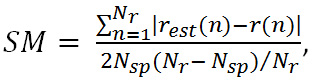, where N_sp and N_r represent respectively the overall spikes count and the length of the response vector; ii)a global measure of fit based on the average response 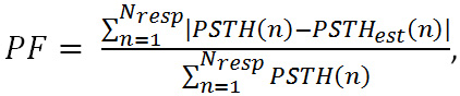where N_resp represents the length of the average response; iii) a measure of model complexity (see also)¹⁰ .

8. Histological Confirmation

1. Sacrifice the rat.
   1. At the end of experimental recordings, put the animal under deep gaseous anaesthesia (Isoflurane 2%, 4 L/min) and inject intravenously a barbiturate overdose (>50 mg/kg, pentobarbital).
   2. Wait the heart arrest.
   3. Unmount the rat from the stereotaxic apparatus
2. Perfusion.
   1. Place the rat laying over a grid onto a basin to collect the blood and fluids from the perfusion.
   2. Open the thorax by dissecting the sternum separating from the rib insertions.
   3. Block the sternal xyphoid process with a cocker forceps and overturning cranially the sternum and divaricate the ribs over the heart.
   4. Identify the left ventricle and the right atrium, place a nine gauge blunted tip needle (connected to the perfusion cannula) into the ventricle and open with surgical fine scissors the right atrium.
   5. Start the perfusion with cold (4 °C) heparinized physiological solution (250 ml) followed by the perfusion of a 4% formalin solution (250 ml).
3. Extract the brain from the skull by opening the cranial vault with a suitable forceps and place the brain in a 10% formalin solution.
4. After a week, prepare the histological slices by a microtome (10 μm thickness).
5. Stain the brain coronal and sagittal sections with cresyl violet solution.

Results

Tip excursion features

To characterize the dynamical properties of the proposed stimulating device, a series of experiments were set up. A specific device which consists of a gallium arsenide infrared emitting diode coupled with a silicon phototransistor was used to assess the tip displacement, the displacement duration and the possible displacement delays. By means of this optical interrupter switch we placed the stimulator tip on the edge of the emitting diode hole (height = 1 mm) and both the microcontroller and the phototransistor outputs were recorded. The placing procedure was facilitated by a microstepper device with a maximum resolution of 1 mm.

The response of devices are shown in Figure 2A. The red line represents the phototransistor response followed by the microcontroller response which indicates the exact beginning of the tip displacement. Notably, a systematic delay due to commutations was present and quantified (Figure 2B, mean = 583 μsec in 100 trials) resulting as abundantly below the desired time precision (1 msec). Finally, we measured the tip displacement duration that was of 3.96 msec on average as shown in Figure 2C.

Randomized Paired Pulse Protocol to Capture LFP and Spike Relations

In order to understand the relation between LFP and spikes, we first set out to generate a stimulation device that can evoke fast and reliable responses from both signals. The Figure 3A shows the inter-stimulus-interval distribution, ensuring that the device provoked a modulation of the spiking activity. The device description and functioning is detailed in the Protocol section.

In Figures 3B and 3C the LFP and spike responses for a representative neuron are shown, respectively. By measuring Mutual Information for spikes and SNR for LFPs (Figures 4A and 4B) it was clear that both encode a substantial amount of information about stimulus occurrence.

Interestingly LFPs and spikes also provided information about the stimulation history (Figures 4C-E). In particular LFP responses were substantially reduced when the actual stimulus was preceded by a previous impulse with a small enough inter-stimulus-interval (Figures 4C and 4D). Neuronal coding of stimulation history positively correlated with MI although exhibited substantially lower values (Figure 4E).

We then asked which features of the LFP signal better correlate with the spike response. After a preliminary analysis, three LFP features that strongly correlate with the average spike response were identified: the average LFP, its derivative and the phase of the LFP derivative (Figure 4F).

A Multi-objective Strategy for Spike Prediction Based on LFPs

Spike trains typically have complex temporal structures that exhibit significant correlations on several timescales. So, which aspects of the neuronal response are captured by LFPs?

A good test to probe the comprehension of the LFP-spike relation is to ask how well spikes are predictable just by looking at the LFP signal. Therefore, by using the above set of LFP features (see Figure 4F), the aim was to build a predictive model that, at any time, reads the values of these features and generates a binary prediction about the occurrence of a spike.

A critical problem related to the fitting of a spike prediction model is constituted by the choice of an appropriate objective function. The most common choices are the Pearson coefficient and the coherence function⁵. Interesting alternatives are provided by spike metrics⁶. While the first two measures are based on the average neuronal responses and therefore do not capture the full structure of the spike trains, the latter is computationally demanding and not practical for fitting purposes. An alternative solution based on multi-objective optimization is proposed. The idea is to jointly minimize more objectives functions (hereafter just called objectives). These objectives have to be computationally efficient to calculate and able to capture different aspects of the neuronal response.

By using the concept of Pareto optimality we can then find a set of models, each optimized for specific trade-offs between these objectives. In order to estimate the Pareto optimal surfaces the NSGAII algorithm was used¹². We identified three objective functions: a global one based on the distance in the average responses, a local one based on the distance on a trial-to-trial basis and an additional objective that penalizes the complexity of the model (see the relative Protocol section).

The results obtained by fitting a representative neuron from our dataset are shown in Figures 5A and 5B. Figure 5A reports the global distance (PF) and the local distance (SM) between model and true responses. Note that the distances for each model are optimal in a Pareto sense so that no model is better or worse than any other one in both distances. The same principle holds for all the three distances jointly considered (Figure 5B).

A main advantage given by the estimation of a set of optimal models instead of a single one lies in the fact that different models, based on optimal trade-offs among the specified objectives, capture different aspects of the true neuronal response. This is shown in Figure 6, where the original raster diagrams (Figures 6A and 6D) and the predicted ones (Figures 6B, 6C, 6E, and 6F) are reported, from two representative neurons: models that minimize the local distance capture the most reliable phase of the neuronal responses (Figures 6B and 6E) while models based on a reasonable trade-off between the local and the global distance better capture the neuron variability and spontaneous firing over the whole temporal range (0-50 msec, Figures 6C and 6F).

Figure 1. (A) Schematic of driver circuit. The main component is an L293D h-bridge. The microcontroller commands are delivered at pins D1 and D2. (B) Blunted tip movements for light mechanical stimulation. The grid size on the graph paper is 1 mm. Click here to view larger image.

Figure 2. Tip displacement features. (A) The outputs of the microcontroller (blue line) and of the phototransistor (red line). The green vertical line is set to 0 indicates the onset of the tip displacement. (B) The probability distribution of the effective tip displacement delays obtained over 100 trials. (C) The probability distribution of the duration of the tip displacement on average in 100 trials. Click here to view larger image.

Figure 3. (A) Inter-Stimulus-Interval distribution. (B, C) "on air" stimuli do not evoke responses (see the top of both graphs in the range 1,000 to 1,200 trials). Compare them to the true stimulus trial run (on the ordinate axes) from 0 to 1,000, where between 15- 40 msec of delay from the stimulus onset (time 0 on the abscissa) clear responses can be observed. The plot in (B) refers to the LFP response whereas the plot in (C) refers to the spike response. In the y-axis of the right most figure, there are the positions ("BIG TOE", "II", "III", etc.) of the stimuli on the hind limb of rats. Click here to view larger image.

Figure 4. (A, B) Mutual Information and LFP_SNR as a function of time along different digits. (C) LFP normalized values after short (<100 msec) and long (>300 msec) Inter-Stimulus-Interval (IStimI). (D) Average Power of the LFP responses after long and short IStimI. Each dot represents a distinct recording. (E) MI about long/short IStimI as a function of the largest MI values about stimulus occurrence (Imax). Each dot represents a distinct neuron. (F) The PSTH of a representative neuron well correlates with three features of the LFP response: the average raw signal, the average derivative and the phase of the derivative. Click here to view larger image.

Figure 5. (A, B) Local and Global distance between predicted and true responses for a representative neuron. (B) Joint evaluation for the three distances. Pareto optimal solutions were estimated by using the NSGAII algorithm. Click here to view larger image.

Figure 6. True (A,D) and estimated (B,C and E,F respectively) responses for two representative neurons. x, y, z respectively represent the raw LFP signal, its derivative and the phase of its derivative. Click here to view larger image.

Discussion

This work firstly presented a new, simple and low-cost device enabling to deliver fast and spatially point-like sensory stimuli. Then a randomized paired pulse stimulation protocol and a set of computational analyses were validated. The overall aim was to establish a framework for the estimation of LFP-spike relations in electrophysiological recordings during tactile stimulation.

The device, the protocol and the analytical approach have jointly contributed to the result, namely the first demonstration of a deterministic approach able to describe and predict LFP-to-spike transitions, a neural process still poorly understood¹.

A critical point was represented by the appropriate setting of the programmable microcontroller board, which regulates strength and length of the tip excursion pulled by the dust-cap. A suitable solution allowing for reliable high frequency stimuli and relatively large displacements has been described in the Results section. Compared to conventional piezoelectric actuators the device provided two main advantages: it escaped the typical problem of mechanical resonance and it allowed relatively large tip displacements.

Neurons in S1 cortex are known to express large receptive fields and fast responses to tactile stimulation⁸. The fast, impulse like stimuli are optimally suited to recruit both superficial and deep skin receptors (e.g. Merkel or Pacinian corpuscles)², and opportunely changing the stimulus parameters (intensity, duration, ramp derivate) one could preferentially recruit one of these different receptor classes. The randomized paired pulse protocol was aimed at reducing predictive entrainment of neuronal oscillations to stimulus occurrence that typically occurs during periodic stimuli. On the other hand the variable interval between the paired pulses allowed us to extract a clear dependence on stimulation history. For the estimation of structure and parameters of our predictive model we relied on a well-known multi-objective optimization algorithm, called the Non-Dominated Sorting Genetic Algorithm II or NSGAII¹². A main problem in fitting a predictive model for spike occurrence relies in the complex temporal structure of real spike trains. Measuring the distance between predicted and true spike trains has proven to be a computationally expensive task⁶. The use of NSGAII, a multi-objective optimization algorithm, allows for breaking down the problem into multiple, computationally efficient distances.

To evaluate the goodness of a model we needed to quantify the error in prediction represented by the distance between predicted and true spike trains. Two main criteria to evaluate model predictions were taken into consideration. The fitting process returned a set of models instead of a single one. Interestingly each model in the set seemed to capture different aspects of the original spike trains.

In conclusion, the developed framework, based on jointly optimized stimulation device, protocol and analyses, could be used to gain further insights into the LFP-spike relation and to ameliorate current strategies for programming efficient brain-machine interfaces and neuroprosthetics.

Materials

List of materials used in this article

Name	Company	Catalog Number	Comments
Microstepper	AB Transvertex (Stockholm, Sweden)		The microstepper used to pull down the electrode matrix
32-channel Cheetah System	Neuralynx (MT, USA)		The electrophysiological recording system
L293D h-bridge	RS Components (Cinisello Balsamo, Italy)		The bridge used to connect the microcontroller to the speaker
H21A3 Optical Interrupter Switch	Fairchild Semiconductor Corporation (San Jose, California)		The phototransistor used to estabilish the tip displacement
Arduino Uno	Arduino (Duemilanove, Italy)		The microcontroller used to deliver current pulse to the speaker
Microelectrode Matrices GB1	FHC
Isoflurane	Rhodia Organique Fine Ltd.		The anesthetic used to prepare animals
Stereotaxic apparatus	Narishighe (Tokyo, Japan)
Sprague-Dawley male rats	Charles River (Calco, LC, Italy)
Gallamine thriethiodide	Sigma-Aldrich		The compound used to curarize the animals
Cresyl violet	Sigma-Aldrich
Topical antiseptics (Betadine 10%)	Meda Pharma (Milanm Italy)
Heparine	Sigma-Aldrich
Formaldehyde	Carlo Erba Reagents (Pomigliano Milanese, Milan, Italy)

References

- Pesaran, B. Uncovering the Mysterious Origins of Local Field Potentials. Neuron. 61 (1-2), (2009).
- Delmas, P., Hao, J., Rodat-Despoix, L. Molecular Mechanisms of Mechanotrasduction in Mammalian Sensory Neurons. Nat. Rev. Neurosci. 12, 139-153 (2011).
- Rasch, M. J., Gretton, A., Murayama, Y., Maass, W., Logothetis, N. K. Inferring spike trains from local field potentials. J. Neurophys. 99 (3), 1461-1476 (2008).
- Galindo-Leon, E. E., Liu, R. C. Predicting stimulus-locked single unit spiking from cortical local field potentials. J. Comput. Neurosci. 29 (3), 581-597 (2010).
- Theunissen, F. E., David, S. V., Singh, N. C., Hsu, A., Vinje, W. E., Gallant, J. L. Estimating spatio-temporal receptive fields of auditory and visual neurons from their responses to natural stimuli. Network. 12 (3), 289 (2001).
- Victor, J. D., Purpura, K. Metric-space analysis of spike trains: theory, algorithms, and application. Network. 8, 127-164 (1997).
- Foffani, G., Chapin, J. K., Moxon, K. A. Computational Role of Large Receptive Fields in the Primary Somatosensory Cortex. J. Neurophysiol. 100 (1), 268-280 (2008).
- Microcontroller website. , Duemilanove, Italy. Available: http://arduino.cc (2014).
- Panzeri, S., Senatore, R., Montemurro, M. A., Petersen, R. S. Correcting for the sampling bias problem in spike train information measures. J. Neurophysiol. 98, 1064-1072 (2007).
- Storchi, R., Zippo, A. G., Caramenti, G. C., Valente, M., Biella, G. E. M. Predicting Spike Occurrence and Neuronal Responsiveness from LFPs in Primary Somatosensory Cortex. PLoS ONE. 7 (5), (2012).
- Quiroga, R. Q., Nadasdy, Z., Ben-Shaul, Y. Unsupervised Spike Detection and Sorting with Wavelets and Superparamagnetic Clustering. Neural Comput. 16, 1661-1687 (2004).
- Deb, K., Agrawal, A., Pratab, A., Meyarivan, T. A fast elitist non-dominated sorting genetic algorithm for multi-objective optimization: NSGA-II IEEE. Trans. Evol. Comput. 6 (2), 181-197 (2000).
Access restricted. Please log in or start a trial to view this content.
Reprints and Permissions