The Measurement of Unsteady Surface Pressure Using a Remote Microphone Probe

Summary

Here, we present a protocol to measure, with high spatial resolution, the unsteady surface pressure in turbulent flows. This method demonstrates the construction of a remote microphone probe (RMP) and the determination of its frequency-dependent, complex transfer function. An analytical determination of the dynamic response is presented and validated.

Abstract

Microphones are widely applied to measure pressure fluctuations at the walls of solid bodies immersed in turbulent flows. Turbulent motions with various characteristic length scales can result in pressure fluctuations over a wide frequency range. This property of turbulence requires sensing devices to have sufficient sensitivity over a wide range of frequencies. Furthermore, the small characteristic length scales of turbulent structures require small sensing areas and the ability to place the sensors in very close proximity to each other. The complex geometries of the solid bodies, often including large surface curvatures or discontinuities, require the probe to have the ability to be set up in very limited spaces. The development of a remote microphone probe, which is inexpensive, consistent, and repeatable, is described in the present communication. It allows for the measurement of pressure fluctuations with high spatial resolution and dynamic response over a wide range of frequencies. The probe is small enough to be placed within the interior of typical wind tunnel models. The remote microphone probe includes a small, rigid, and hollow tube that penetrates the model surface to form the sensing area. This tube is connected to a standard microphone, at some distance away from the surface, using a "T" junction. An experimental method is introduced to determine the dynamic response of the remote microphone probe. In addition, an analytical method for determining the dynamic response is described. The analytical method can be applied in the design stage to determine the dimensions and properties of the RMP components.

Introduction

Fluid flow over surfaces generally leads to unsteadiness and turbulence that result in unsteady surface pressure (USP). Flow-induced sound and vibration are often a direct result of this unsteadiness. The radiated sound generated by cooling fans, propellers, and wind turbines are dominated by sources related to USP¹. Measurements of the spatial and temporal characteristics of USP in turbulent flows are generally required in order to predict the radiated sound.

The statistical characterization of USP is generally given in the form of auto-spectral density, two-point cross-spectral densities, and spatial correlation functions^{2, 3}. The frequency response required can vary depending on the application. In many wind tunnel applications, a response of 10 kHz to 20 kHz is sufficient. The small scales of turbulent motion often require sensing areas and sensor spacing to be less than 1 mm.

Extensive experimental studies have been conducted in order to obtain turbulence-induced pressure fluctuations. A direct method uses flush-mounted embedded sensors. This method often employs large arrays of microphones, because each sensor can only measure the pressure fluctuation at one discrete point. Typical sensors utilized in this method are piezoelectric transducers, suggested by Gautschi⁴. Arrays of piezoelectric sensors can be expensive, and the frequency range of measurement is often less than 10 kHz.

Direct surface-mounted microphones are often used as inexpensive USP sensors⁵. Microphones have high sensitivity, which is a substantial benefit for low-speed flows. However, this also leads to the risk of sensor saturation when large amplitude fluctuations in pressure are present. This method is not suitable for surfaces with large curvatures, discontinuities, or geometries that are too thin to contain the entire sensor.

An indirect method for obtaining both spectral and spatial information is to use thin membranes flush-mounted to a surface⁶. The time- and space-dependent vibration motions are measured and then converted to surface pressure statistics using known mechanical properties of the membrane. This method requires careful design, implementation, and accurate calibration of the membrane's dynamic response. Additionally, the vibration measurement equipment, such as laser Doppler vibrometers, are expensive. Lastly, this method can only be applied to flat surfaces.

Pressure-sensitive paint (PSP) is another technique that can be used to measure the unsteady surface pressure. This technique requires the surfaces to be coated in a transparent polymer binder, which causes the molecules within to be excited to a higher energy state as they are illuminated by light of a specific wavelength. As the molecules undergo oxygen quenching, energy is released as light at a rate proportional to the oxygen partial pressure, resulting in luminescence that is inversely proportional to the surface pressure⁷. The major drawback to PSP methods is the relatively low sensitivity of the measurement when compared to microphones. This limits the application of PSP to relatively high-speed flows.

The present communication describes a method for USP that uses a remote microphone probe (RMP). This method was first described by Englund and Richards⁸. The concept uses a standard miniature microphone that is connected to the surface pressure tap with a hollow tube. The unsteady pressure at the model surface will travel into the tubing in the form of sound waves. The tubing acts as a "wave-guide" to allow the microphone, which is mounted perpendicularly to the tubing, to measure the sound waves. The waves then continue into another tube that is long enough to eliminate large-amplitude acoustic reflections.

Englund and Richards applied an analytical approach outlined by Bergh and Tijdeman⁹ to determine the dynamic response of the RMP. Perrenes and Roger¹⁰ utilized an RMP to measure surface pressure over a two-dimensional airfoil with high-lift devices. They developed a probe with a 0.5 mm diameter capillary tube at the surface that was connected to a 27-cm-long rigid tube that expanded from 0.7 mm to 2.5 mm via two separate step changes. Each step change caused a relatively large change in the acoustic impedance of the tube. Leclercq and Bohineust¹¹ studied the wall pressure field beneath a turbulent boundary layer. They used a constant-diameter RMP, as suggested by Franzoni and Elliott¹². However, the dynamic response was high enough only in a limited frequency range. Arguillat et al.¹³ designed an RMP to study the noise transmitted to the interior of a vehicle compartment. They tested various tubes to conduct the pressure fluctuation to the microphones. Yang et al.¹⁴ corrected for the tubing distortion by using a tubing transfer function approach that is similar to the method introduced in this report. Hoarau et al.¹⁵ studied the wall pressure trace downstream of a separated region. The RMPs that they designed had constant inside diameters, and the tubing was entirely non-rigid.

According to previous studies, the accuracy of surface pressure measurements obtained using RMPs is mainly dependent upon the determination of the frequency-dependent transfer function of the probe that relates the surface pressure to the microphone pressure. The following sections will describe an RMP geometry that is both simple and effective. Experimental and analytical methods will be introduced and validated in order to accurately determine the dynamic response of the RMP. The analytical model allows for an RMP to be optimized in the design stage for a potentially wide range of applications.

RMPs can be used to measure pressure fluctuations over a wide range of frequencies. The relatively high spatial resolution can offer detailed information on characteristics of the spatially-distributed unsteady pressure field¹⁶. As the probe is small, RMPs can be utilized to measure pressure fluctuations over complex geometries, such as large curvatures or limited spacing¹⁷. In addition, the tube connecting the surface tap and the microphone sensor can reduce the magnitude of the induced pressure fluctuation at the microphone. Thus, proper design of RMP sensor geometry and parameters yields a method for obtaining USP characteristics that are significantly less restrictive when compared to flush-mounting the microphone directly to the model surface.

Structure of the RMPThe general structure of the RMP is shown in Figure 1. The RMP consists of one tube leading from the model surface to an expansion section and a second tube extending from the expansion section to a "cradle." A third tube is then connected to act as an anechoic termination. The cradle is a machined plastic component used for housing the microphone and the tube connections. The details of the RMP structure can be adjusted for various experimental conditions. The purpose of the second, larger-diameter tube is to allow the relatively bulky microphone and cradle to be placed further from the point of the USP measurement without significantly reducing the measurement sensitivity. This second tube can be eliminated if it is not necessary, and the expansion section can be built in the cradle. The anechoic termination was made of soft plastic that was approximately 2 to 3 m in length.

For this demonstration, the design of the RMP was optimized for the measurement of surface pressure fluctuations under a turbulent boundary layer without a streamwise pressure gradient, as shown in Figure 2. The second tube was eliminated. The effects of the two different lengths of the first tube were observed. The first tube was constructed from stainless steel with an inner diameter of 0.5 mm and an outer diameter of 0.81 mm. The lengths of the first tube were 5.35 and 10.40 cm, respectively. The inner diameter of the inlet of the expansion section, which was incorporated into the cradle, was 0.5 mm, and the inner diameter of the exit was 1.25 mm, which was identical to the inner diameter of the dissipation termination. The angle of the expansion section was 7°. There was a hole in the cradle with a 1.25 mm diameter in order to smoothly connect the expansion section with the anechoic termination. The sensing area was connected to the 1.25 mm hole through a perpendicular 0.75 mm hole.

Protocol

1. Preparation of Experiments

1. Select a proper microphone to build the RMP. Use a frequency range of the microphone within the frequency range of interest.
   NOTE: In this experiment, pressure fluctuations between 100 and 10,000 Hz are of interest. The measurement frequency range of the selected microphone is from 100 to 10,000 Hz. The size of the microphone should be as small as possible, although there are no specific criteria for the size.
2. Estimate the sensitivity and frequency response of the RMP system using the analytical method described in the appendix. Adjust the sensitivity and frequency response of the RMP by varying the dimensions of the tubes and structures.
3. Use a Dremel to cut the 0.5 mm inner-diameter stainless steel tube into a 5.25 cm long piece.
4. With scissors, cut the 1.25-mm inner-diameter soft tube into a 4.75 m long piece.
5. Use a milling machine to cut a piece of Plexiglas into a cuboid. The length, width, and height of the cuboid should be 2.54 cm, 1.27 cm, and 1.27 cm, respectively.
6. Drill holes with 0.81, 2, 2.56, and 0.76 mm diameters on the Plexiglas cradle, as shown in Figure 2.
7. Use a needle drill to make the taper section of the Plexiglas cradle, as shown in Figure 2.
8. Look up the microphone sensitivity in the manual provided by the manufacturer, or calibrate the microphone using the method introduced by Wong¹⁸.
9. Seat the microphone into the Plexiglas cradle, as shown in Figure 2, and fix the microphone using epoxy.
10. Connect the stainless-steel tube and the soft tube to the Plexiglas cradle and fix them with epoxy.
11. Drill a hole with a 0.81 mm diameter perpendicularly to the model surface at the position of measurement.

2. Experiment Setup

1. Flush mount the primary stainless steel tubes of the RMP sensors to the model surface and add epoxy to fix the stainless steel tubes to the opposite model surface, as shown in Figure 2.
2. Surround the RMP with acoustic foam in order to prevent parasitic noise from contaminating the system.
3. Route all electrical wiring out of the test section of the tunnel.
4. Route the soft anechoic tube out of the test section of the tunnel.
5. Connect the end of the soft anechoic tube to a pressure transducer in order to obtain measurements of the mean static pressure simultaneously with the unsteady pressure.
6. Connect the RMP to a low-noise amplifier and data acquisition system.
7. Set the gain factor of the amplifier to 10. Note that the value of the gain factor can be changed from case to case.

3. Calibration

1. Select a reference microphone that is high quality and has a frequency-independent sensitivity.
2. Connect the reference microphone to the input of an amplifier and connect the output of the amplifier to the data acquisition system.
3. Set both the input gain and output gain of the amplifier to 10 dB. Note that the gain factor can be varied under different measurement conditions.
4. Insert the reference microphone into a pistonphone, as shown in the supplementary figure.
5. Turn on the pistonphone.
6. Set the acquisition frequency to 4,000 Hz.
7. Set the number of samples to 240,000.
8. Acquire and save the voltage output from the reference microphone.
9. Compute the calibration constant of the reference microphone. The calibration constant, C_ref, is the ratio of the standard deviation of the pistonphone-produced sound pressure to the standard deviation of the voltage output of the reference microphone.
10. Repeat the calibration process (steps 3.8 and 3.9) several times. Use the mean value, C_ref, as the calibration constant.
11. Place the reference microphone perpendicularly to the solid surface over which the pressure fluctuation is measured, as shown in Figure 1.
12. Align the center of the reference microphone with the RMP tap. Use a distance between the reference microphone and the RMP tap of 1 mm.
13. Place the loudspeaker in close proximity to the test model. Use a distance between the loudspeaker and the microphone of 2.5 m for these measurements.
14. Connect the loudspeaker to a function generator and turn on the function generator.
15. Use the "white noise" option of the function generator to provide the desired acoustic signal and set the root mean square voltage, V_rms, to 0.4 V.
16. Adjust the volume of the loudspeaker to the minimum.
17. Turn on the loudspeaker.
18. Adjust the volume of the loudspeaker amplifier as high as possible without damaging the speaker. Note that most speakers have an indicator light to warn the user if the output amplitude is above the speaker range.
19. Acquire and save time-series data from the voltage outputs of both the reference microphone and the RMP using a scanning frequency of 40,000 Hz for 60 sec.
20. Compute the time-series values of the sound pressure fluctuation, which is generated by the loudspeaker and function generator and measured by the reference microphone. This is simply the product of the time-series voltage output from the reference microphone, , and its calibration constant, ; . Note that the time-series sound pressure, , is also the pressure fluctuation at the tap of the RMP.
21. Compute the time-series sound pressure fluctuation measured by the microphone in the RMP as the product of the time-series voltage output from the RMP, , and the microphone sensitivity, ; . Note that the microphone sensitivity, , should be provided by the manufacturer.
22. Compute the auto-spectral density, , of  . Compute the auto-spectral density, , of . Compute the cross-spectral density, , between and . The auto-spectral densities and cross-spectral density are defined by Bendat and Piersol¹⁹.
23. Compute the transfer function as .
24. Compute the coherence function as , where the asterisk represents the complex conjugate.
25. Remove the reference microphone.
26. Turn off the loudspeaker and function generator.
27. Remove the loudspeaker.

4. Data Acquisition

1. Turn on the wind tunnel.
2. Record the time-series voltage output, , of the RMP with the data acquisition system. Use a scanning frequency of 40,000 Hz. Use a duration of the acquisition of 64 sec.
3. Turn off the wind tunnel.

5. Data Processing

1. Compute the sound pressure fluctuation, , measured by the microphone in the RMP as .
2. Compute the auto-spectral density, , of the surface pressure fluctuation as , where is the auto-spectral density of the sound pressure fluctuation measured by the microphone in the RMP .

Representative Results

Calibration results from two representative RMP designs are shown in this section. The first one used a 5.35 cm primary tube, and the second one used a 10.4 cm primary tube. The dissipative terminations are 4.75 m long for both RMPs.

The coherence between the pressure fluctuations measured by the microphone in the RMP and by the reference microphone is shown in Figure 3. The data show a near-unity coherence value over a wide range of frequencies. At frequencies above 10 kHz, the coherence generally remains high, but the coherence drops intermittently at some frequencies. One reason for this is that the sound generated by the loudspeaker is comparatively low at these frequencies. This may also result from the reduced sensitivity of the RMP at high frequencies. The background and electrical noise can result in the loss of coherence. A low coherence value indicates that the pressure fluctuations measured by the microphone in the RMP and the reference microphone are not strongly correlated. In this study, the coherence is higher than 0.97 in the frequency range of interest.

Figure 4 shows the magnitude of the transfer function obtained both experimentally and analytically. The analytical method is accurate in predicting the dynamic response across most of the frequency range. The disagreements in the middle- and high-frequency ranges are assumed to be a result of small aberrations in the RMP, such as burs or slight mismatches at tubing junctions.

The oscillations in the transfer function magnitude at frequencies between 100 Hz and 500 Hz are related to acoustic reflections in the longer anechoic termination. These are generally on the order of 1 or 2 dB in magnitude. Acoustic reflections within the primary tube are evident in the oscillations at higher frequencies.

Figure 5 shows the phase shift of the transfer functions. The analytical method slightly overestimates the slope of the phase shift. Although the uncertainty of the measurement, which is about 1.6%, can result in discrepancy, this overestimation is considered to be caused by small errors in estimated tube lengths or by temperature variations, which will affect the acoustic speed applied in the analytical method because of the constant trend.

USP measurements were acquired in a flat-plate turbulent boundary layer flow. This method was chosen for this communication because of the simplicity of the experimental setup and because a significant body of data for the USP exists for the flat-plate boundary layer. The auto-spectral densities measured by the RMP at several values of the Reynolds number are shown in Figure 6. The pressure spectra were normalized by wall shear, displacement thickness, and uniform flow speed. The light gray region contains all of the data from various research groups, compiled by Goody²⁰. The dark grey band represents pressure spectra that correspond to very large Reynolds numbers. The present measurements are within the spread of measurements observed in previous literature and demonstrate the anticipated trend of the magnitude decreasing with the Reynolds number, as shown by Goody. Note also that the measured pressure spectra do not contain any of the harmonic peaks that exist in the transfer function, indicating that an accurate frequency-dependent calibration function was applied.

Figure 1: Schematic for RMP structure and setup. The schematic shows the general design of the RMP. The details of the RMP can be adjusted to optimize the design for various measurement conditions. Please click here to view a larger version of this figure.

Figure 2: The dimensions and setup of the RMP utilized to measure the surface pressure under the canonical turbulent boundary layer in the present study. The design of the RMP utilized for this measurement is slightly different from the structure shown in Figure 1; the expansion section is incorporated into the cradle. Please click here to view a larger version of this figure.

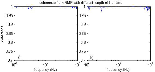
Figure 3: Coherence functions for RMPs with various first-tube lengths. (left) 5.35 cm first tube and (right) 10.40 cm first tube. The x-axis is the frequency in Hz, and the y-axis is the value of the coherence. Please click here to view a larger version of this figure.

Figure 4: Magnitude of the transfer functions for RMPs with various first-tube lengths. (left) 5.35 cm first tube and (right) 10.40 cm first tube. The blue curve represents the experimental results, while the green curve represents the theoretical predictions. The x-axis is frequency in Hz, and the y-axis is the magnitude of the transfer function in dB. Please click here to view a larger version of this figure.

Figure 5: Phase shift of the transfer functions for RMPs with various first-tube lengths. (left) 5.35 cm first tube and (right) 10.40 cm first tube. The blue curve represents the experimental results, and the green curve represents the theoretical predictions. The x-axis is frequency in Hz, while the y-axis is the phase shift of the transfer function in rad. Please click here to view a larger version of this figure.

Figure 6: Auto-spectral density of the surface pressure measured by RMPs under various Reynolds numbers. The x-axis represents the angular frequency, normalized by displacement thickness and uniform flow speed; the y-axis shows the surface pressure spectra, normalized by uniform flow speed, displacement thickness, and wall shear. Please click here to view a larger version of this figure.

Discussion

The measurement of USP in wind tunnel experiments is needed for many applications related to aeroacoustics and flow-induced vibrations. Compared to existing methods, such as flush-mounted imbedded sensors, PSP, or vibrated membranes, the method described here allows for accurate measurements with a high sensitivity to large-magnitude fluctuation over a wide range of frequencies. More importantly, it also provides a method for USP measurements using a small sensing area that minimizes the spatial averaging effects described by Corcos²¹. Additionally, the method allows for the close spacing of sensors over complex geometries. While RMP designs have been proposed in past literature, this communication provides details regarding an effective RMP design methodology, along with a theoretical method for choosing the parameters required for an effective measurement.

The analytical method can predict the dynamic response of the RMP in the design stage. As shown in the representative results, the frequencies of the resonance maxima are determined by the length of the first tube. As a result, the length of the first tube can be adjusted in order to position the resonance peak at a desired frequency. For example, if the magnitudes of the surface pressure fluctuations at certain frequencies are anticipated to be large, the length of the first tube should be adjusted to ensure that the resonance peak is not located at those frequencies.

The most critical step for the application of the RMP system is the calibration. The coherence function is an indication of the calibration quality. High coherence is always desired. However, the coherence function can be affected by several parameters, including the frequency, range, and acoustic amplitude of the loudspeaker; the relative location of the loudspeaker; the distance between the reference microphone and the tap of the RMP; and the dimensions of the tubing in the RMP. The effects of the aforementioned parameters on the calibration are complicated. Even now, there is no optimized method for determining all of these parameters. The calibration process should be repeated to obtain the best coherence value.

The structure of this RMP system can be modified based on the predictions of the analytical method in the design stage to account for various experimental conditions. Therefore, this RMP technique can be optimized and applied to the measurement of surface pressure fluctuation under complex flow conditions, such as the unsteady surface pressure present in turbomachinery.

Materials

Name	Company	Catalog Number	Comments
Microphone	ACO Pacific (http://www.acopacific.com/)	7016	Used to measure the sound pressure and calibrate the RMP as a reference.
Microphone	Knowles (http://www.knowles.com/eng)	FG-23629-C36	Used to measure the pressure fluctuation as a part of the RMP.
Microbore Tubing	Saint-gobain (http://www.biopharm.saint-gobain.com/en/index.asp)	Tygon ND 100-80	Used to dissipate the sound waves as a dissipation termination.
Hypodermic Tubing	MicroGroup (http://www.microgroup.com/)	304H21RW	Used to connect the surface tap and allow the surface pressure fluctuation to convect to the microphone in the RMP in the form of sound.
Hypodermic Tubing	MicroGroup (http://www.microgroup.com/)	304H14H	Used to reduce the dissipative effect and allow the surface pressure fluctuation to convect to the microphone in the RMP in the form of sound.
plexiglass	Plaskolite (http://www.plaskolite.com/)	1X76204A	Used to make cradles which can connect the tubing and the microphone for the RMP.
Data acquisition chassis	National Instruments (http://www.ni.com/)	PXI-1006	For data acquisition.
Data acquisition channel	National Instruments (http://www.ni.com/)	PXI-4472	For data acquisiton.
Function generator	thinkSRS (http://www.thinksrs.com/)	DS360	To generate white noise signal.
Pistonphone	B&K (http://www.bksv.com/)	4228	To generate sine waves with constant frequency which will be used to calibrate the reference microphone.
Loudspeaker	Mackie (http://www.mackie.com/index.html)	HD1531	Used to convert the electrical white noise signal into sound. It is the sound source for calibrating the RMP.
MatLab	Mathworks (http://www.mathworks.com/)		Used to process experimental data.
LabVIEW	National Instruments (http://www.ni.com/)		Used control the hardware for data acquisition and record the data.

References

- Blake, W. K. Mechanics of Flow-induced sound and vibration. , Academic Press. Orlando, FL. (1986).
- Schloemer, H. Effects of pressure gradients on turbulent-boundary-layer wall-pressurefluctuations. J Acoust Soc Am. 42 (1), 93-113 (1967).
- Willmarth, W., Wooldridge, C. Measurements of fluctuating pressure at wall beneath a thick turbulent boundary layer. J Fluid Mech. 14 (2), 187-210 (1962).
- Gautschi, G. Piezoelectric Sensorics: Force, Strain, Pressure, Acceleration and Acoustic Emission Sensors, Materials and Amplifiers. , Springer. Berlin. (2002).
- Blake, W. K. A statistical description of pressure and velocity fields at the trailing edges of a flat strut. , David W. Taylor Naval Ship Research and Development Center. Report 4241 (1975).
- Huettenbrink, K. B. Lasers in Otorhinolaryngology. , Thieme. (2005).
- Bell, J. H., Schairer, E. T., Hand, L. A., Mehta, R. D. Surface Pressure Measurement using Luminescent Coatings. Annu Rev Fluid Mech. 33, 155-205 (2001).
- Englund, D., Richards, W. The infinite line pressure probe. ISA Transactions. 24 (2), 11-19 (1985).
- Bergh, H., Tijdeman, H. Theoretical and Experimental Results for the Dynamic Response of Pressure Measuring Systems. NRL Report TR F 238. National Aero-and Astronautical Research Inst. , Amsterdam. (1965).
- Perennes, S., Roger, M. Aerodynamic noise of a two-dimensional wing with high-lift devices. 4th AIAA/CEAS Aeroacoustics Conference, , Toulouse. (1998).
- Leclercq, D., Bohineust, X. Investigation and modeling of the wall pressure field beneath a turbulent boundary layer at low and medium frequencies. J Sound Vibrat. 257 (3), 477-501 (2002).
- Franzoni, L. P., Elliott, C. M. An innovative design of a probe-tube attachment for a half in microphone. JASA. 104, 2903-2910 (1998).
- Arguillat, B., Ricot, D., Robert, G., Bailly, C. Measurements of the wavenumber-frequency spectrum of wall pressure fluctuations under turbulent flows. Collection of Technical Papers - 11th AIAA/CEAS Aeroacoustics Conference. 1, 722-739 (2005).
- Yang, H., Sims-Williams, D., He, L. Unsteady pressure measurement with correction on tubing distortion. Unsteady Aerodynamics, Aeroacoustics and Aeroelasticity of Turbomachines. , Springer. Berlin. 521-529 (2006).
- Hoarau, C., Boree, J., Laumonier, J., Gervais, Y. Analysis of the wall pressure trace downstream of a separated region using extended proper orthogonal decomposition. Phys Fluids. 18 (5), 055107 (2006).
- Bilka, M. J., Paluta, M. R., Silver, J. C. Spatial correlation of measured unsteady surface pressure behind a backward-facing step. EXIF. 56 (2), (2015).
- Probsting, S., Gupta, A., Scarano, F., Guan, Y., Morris, S. C. Tomographic PIV for Beveled Trailing Edge Aeroacoustics. 20th AIAA/CEAS Aeroacoustics Conference, , AIAA Paper (2014).
- Wong, G. Microphones and Their Calibration. Springer Handbook of Acoustics. , Springer. (2007).
- Bendat, J. S., Piersol, A. G. Random data: analysis and measurement procedures. , John Wiley & Sons. New York, NY. 2nd edition (1986).
- Goody, M. Empirical spectral model of surface pressure fluctuations. Am Instit Aero Astronaut. 42 (9), 1788-1794 (2004).
- Corcos, G. M. Resolution of pressure in turbulence. J Acoust Soc Am. 35 (2), 192-199 (1963).
- Tijdeman, H. On the propagation of sound waves in cylindrical tubes. J Sound Vibrat. 39 (1), 1-33 (1975).
- Iberall, A. S. Attenuation of oscillatory pressures in instrument lines. J Res Natl Bureau Stand. 45 (1), 85-108 (1950).
- Zwikker, C., Kosten, C. Sound Absorbing Materials. , Elsevier. Amsterdam. (1949).