Summary
We present a protocol for measuring the thermal properties of synthetic hydrate-bearing sediment samples comprising sand, water, methane, and methane hydrate.
Abstract
Methane hydrates (MHs) are present in large amounts in the ocean floor and permafrost regions. Methane and hydrogen hydrates are being studied as future energy resources and energy storage media. To develop a method for gas production from natural MH-bearing sediments and hydrate-based technologies, it is imperative to understand the thermal properties of gas hydrates.
The thermal properties' measurements of samples comprising sand, water, methane, and MH are difficult because the melting heat of MH may affect the measurements. To solve this problem, we performed thermal properties' measurements at supercooled conditions during MH formation. The measurement protocol, calculation method of the saturation change, and tips for thermal constants' analysis of the sample using transient plane source techniques are described here.
The effect of the formation heat of MH on measurement is very small because the gas hydrate formation rate is very slow. This measurement method can be applied to the thermal properties of the gas hydrate-water-guest gas system, which contains hydrogen, CO2, and ozone hydrates, because the characteristic low formation rate of gas hydrate is not unique to MH. The key point of this method is the low rate of phase transition of the target material. Hence, this method may be applied to other materials having low phase-transition rates.
Introduction
Gas hydrates are crystalline compounds that comprise cage structures of hydrogen-bonded water molecules containing guest molecules in the cage1. Large amounts of methane hydrates (MHs) in the ocean floor and permafrost regions are interesting future energy resources but may affect global climate conditions2.
In March 2013, the Japan Oil, Gas, and Metals National Corporation conducted the world's first offshore production test to extract gas from natural MH-bearing sediments in the eastern Nankai Trough using the "depressurization method" 3,4.
Gas hydrates can store gases such as methane1, hydrogen5, CO21,6, and ozone7. Hence, methane and hydrogen hydrates are studied as potential energy storage and transportation media. To reduce the CO2 emissions released into the atmosphere, CO2 sequestration using CO2 hydrates in deep-ocean sediments have been studied6. Ozone is currently used in water purification and food sterilization. Studies of ozone preservation technology have been conducted because it is chemically unstable7. The ozone concentration in hydrates is much higher than that in ozonized water or ice7.
To develop gas production from natural MH-bearing sediments and hydrate-based technologies, it is imperative to understand the thermal properties of gas hydrates. However, the thermal properties data and model studies of gas hydrate-bearing sediments are scarce8.
The "depressurization method" can be used to dissociate MH in the sediment pore space by decreasing the pore pressure below the hydrate stability. In this process, the sediment pore space components change from water and from MH to water, MH, and gas. The thermal properties' measurement of the latter condition is difficult because the melting heat of MH may affect the measurements. To solve this problem, Muraoka et al. performed the thermal properties' measurement at supercooled conditions during MH formation9.
With this video protocol, we explain the measuring method of supercooled synthetic sand-water-gas-MH sample.
Figure 1 shows the experimental setup for measuring the thermal properties of the artificial methane hydrate-bearing sediment. The setup is the same as shown in reference9. The system mainly comprises a high-pressure vessel, pressure and temperature control, and thermal properties of the measurement system. The high-pressure vessel is composed of cylindrical stainless steel with an internal diameter of 140 mm and a height of 140 mm; its inner volume with the dead volume removed is 2,110 cm3, and its pressure limit is 15 MPa. The transient plane source (TPS) technique is used to measure the thermal properties10. Nine TPS probes with individual radii of 2.001 mm are placed inside the vessel. The layout of the nine probes9 is shown in Figure 2 in reference9. The TPS probes are connected to the thermal properties' analyzer with a cable and switched manually during the experiment. The details of the TPS sensor, connection diagram, and setup in the vessel are shown in Figures S1, 2, and 3 of the supporting information in reference9.

Figure 1: The experimental setup for measuring the thermal properties of the artificial methane hydrate-bearing sediment. The figure is modified from reference9. Please click here to view a larger version of this figure.
The TPS method was used to measure the thermal properties of each sample. The method principles are described in reference10. In this method, the time-dependent temperature increase, ΔTave, is

where

In Equation 1, W0 is the output power from the sensor, r is the radius of the sensor probe, λ is the thermal conductivity of the sample, α is the thermal diffusivity, and t is the time from the start of the power supply to the sensor probe. D(τ) is a dimensionless time dependent function. τ is given by (αt/r)1/2. In Equation 2, m is the number of concentric rings of the TPS probe and I0 is a modified Bessel function. The thermal conductivity, thermal diffusivity, and specific heat of the sample are simultaneously determined by inversion analysis applied to the temperature increase as power is supplied to the sensor probe.
Subscription Required. Please recommend JoVE to your librarian.
Protocol
Note: Please consult all relevant material safety data sheets as this study uses high-pressure flammable methane gas and a large high-pressure vessel. Wear a helmet, safety glasses, and safety boots. If the temperature control system stops, the pressure in the vessel increases with MH dissociation. To prevent accidents, the use of a safety valve system is strongly recommended to automatically release the methane gas to the atmosphere. The safety valve system can work without electrical power supply.
1. Preparation of the Sand-water-methane Gas Samples9
- Place the high-pressure vessel on the vibrating table.
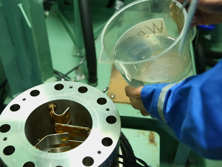
- Pour 1.5 L of pure water in a water bottle and 4,000 g silica sand in a sand bottle. Accurately weigh the masses of sand and water in the sand and water bottles, respectively.
- Pour 1 L of pure water in the high-pressure vessel with an inner volume of 2,110 cm3 from a water bottle until the water fills half the inner vessel.
- Turn on the vibrating table to vibrate the entire vessel. Set the vibration rate and the power supply to 50 Hz and 220 W, respectively. Apply the vibration until the completion of step 1.5. Remove the residual air in the drain line and sintered metallic filter at the bottom of the vessel by vibrating the vessel.
- Pour 3,300 g silica sand from a sand bottle into the vessel at a constant rate of approximately 1 g sec−1 using a funnel held near the water surface while the entire vessel is vibrated to ensure uniform packing.
- Stop the vibration when the water reaches the rim of the vessel.
- Place a ring as a temporary wall on the rim of the vessel to prevent water from spilling.
- Vibrate the vessel again at 50 Hz and 220 W.
- When the sand reaches the rim of the vessel (height 140 mm), turn off the vibration.
- Remove the temporary wall and excess pore water using the drain line. Pour the excess pore water back into the water bottle.
- Pack the sand by vibrating the vessel once or twice at 50 Hz and 300 W for 1 sec and add more sand if necessary.
- Weigh the masses of sand and water in the sand and water bottles. Calculate the sand and water masses in the vessel from the mass differences in the sand and water bottles. In this experiment, the masses of sand and water in the vessel were 3,385 g and 823.6 g, respectively. The mass of water in the vessel is denoted as wtotal.
- Cover the high-pressure vessel with a stainless steel lid and tighten the bolts of diagonally opposite pairs in sequence.
- Move the high-pressure vessel from the vibrating table to the table intended for the experiment.
- Cover the high-pressure vessel with the heat insulator for controlling the temperature.
- Connect the high-pressure pipelines and the cooling water flow lines to the high-pressure vessel.
- Open the valves of the input and output gas pipelines. Ventilate 10 L methane at a rate of 800 ml min−1 until no excess water discharges into the trap under atmospheric pressure. The sand discharge is prevented by a sintered metallic filter fixed on the bottom of the vessel. The residual water remains on the sand surface because the hydrophilic silica sand adsorbs the water molecules.
- Weigh the mass of water in the trap, wtrap, to determine the gas volume in the vessel. Determine the mass of residual water, wres, in the vessel using the equation wres = wtotal − wtrap. In this case, wres and wtrap was 360.6 g and 463.0 g, respectively.
- Determine the sample porosity using the formula Ѱ = 1 - Vsand / Vcell, where Vsand is the volume of the sand determined by the ratio of sand mass to sand density (i.e., ρs = 2,630 kg m−3), and Vcell is the inner volume of the vessel. The porosity Ѱ of the sample was 0.39.
- Close the valve of the output gas line. Inject methane to increase the pore pressure of methane in the vessel to approximately 12.1 MPa at room temperature (i.e., 31.6 °C).
- Close the valve of the input gas line.
- Start recording the pressure and temperature in the vessel during the experiment using the data logger. The data sampling interval is 5 sec. The total experimental time is approximately 3,000 min.
2. MH Synthesis and Thermal Properties' Measurement of the Supercooled Sample9
- Turn on the chiller for cooling the vessel from room temperature to 2.0 °C by circulating the coolant. Let the coolant circulate from the chiller to the bottom of the vessel, from there to the lid of the vessel, and finally back to the chiller. The temperature change rate in the vessel was approximately 0.001 °C sec−1.
- Set the measurement parameters using the TPS analyzer software. Set the sensor type to sensor design #7577. Set the output power W0 to 30 mW and the measuring time to 5 sec. Note that the appropriate parameters should be changed if the sensor type or sample conditions change. Set the parameters to increase the temperature from 1 °C to 1.5 °C.
- Calculate the degree of supercooling, ΔTsup, with the following equation:
ΔTsup = Teq(P) − T. (3)
Teq(P) is the equilibrium temperature of MH as a function of pressure P. Teq(P) is calculated using the CSMGem software1. P and T are the pressure and temperature in the vessel measured by using pressure and temperature gauges, respectively. - Simultaneously measure the thermal conductivity, thermal diffusivity, and volumetric specific heat using the TPS analyzer after ΔTsup is greater than 2 °C.
- Switch the TPS probe connected to the thermal properties analyzer after each measurement. Switch the cables between the TPS probes and the analyzer manually during the experiment9. The connection diagram is shown in Figure S2 in reference9. The switching sequence for each sensor is no. 6 → 2 → 7 → 5 → 1 → 9 → 4 → 3 → 8 → 6…. The sequence is based on the distance between the sensors, which is set as far as possible to prevent the residual heat from affecting the measurements. Collect data every 3-5 min.
- Repeat the measurements until ΔTsup reaches 2 °C again. In this experiment, ΔTsup initially increases with time. After ΔTsup reaches the maximum value, ΔTsup gradually decreases to 0 °C because the pressure decreases with the formation of MH. Check if ΔTsup is greater than 2 °C prior to the TPS measurements using equation 3.
- Ensure that the temperature profile is not affected by MH melting. If MH melts during the measurements, the temperature will not increase because melting of MH is an endothermic reaction. Check the temperature profile during the measurements, and is discussed in the results section.
- Perform the thermal properties' analysis for all temperature profile data using the TPS technique.
3. Calculation of the Saturation Change of the Sample9,11
Note: The degree of saturation for MH, water, and gas in the sample as a function of time t is calculated using the equation of state of the gas. The calculation details and equations used are previously described11.
- Calculate the methane gas volume Vgas,t at time t

where Q is the initial volume of gas in the vessel, VMH,t − 1 is the volume of MH at time t − 1, and RVhw is the volume ratio of water and MH.
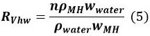
In Equation 5, n is the hydration number of MH (~6), ρMH and ρwater correspond to the density of MH and water, respectively, and wMH and wwater denote the molecular mass of MH and water, respectively. - Calculate the amount ΔMt (mol) of MH formed from t − 1 to t
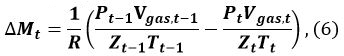
where R is the gas constant, P is the pressure of the methane gas, and Zt (Tgas,t, Pgas,t) is the compression coefficient of methane at time t. We9 and Sakamoto et al.11 have used the Benedict–Webb–Rubin (BWR) equation, as modified by Lee and Kesler, for calculating Zt12,13. For this calculation, the formulas (3–7.1)–(3–7.4) of the BWR equation13 and the Lee–Kesler constants are used in Tables 3–7 of reference13. - Calculate the volume change ΔVMH,t of MH from t − 1 to t

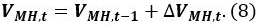
where Ps is the reference pressure of 101325 Pa, Ts is the reference temperature of 273.15 K, Zs is the compression coefficient at Ps and Ts (Zs ~1), and VCH4 is the ratio of the methane gas volume in the unit volume of MH [Nm3 m−3]. Use a VCH4 value of 165.99 [Nm3 m−3]. - Calculate the volume VMH,t of MH at time t
- Calculate the volume of water Vwater,t in the pressure vessel at time t

where Vwater,1 is the initial volume of water. - Repeat the calculations using Equations. 4–9 at time t = 2, 3, … to determine the change in the saturation of water, methane, and MH11. The initial condition is t = 1, i.e., Vgas,1 = Q. The P and T at time t are taken from the data logs9. The calculation results are shown in the following section.


Subscription Required. Please recommend JoVE to your librarian.
Representative Results
Figure 2a shows the temperature profile that is not affected by MH melting. ΔTc is the temperature change due to thermal constants' measurement. Figure 2b shows the temperature profile that is affected by MH melting. The profile in Figure 2b cannot be analyzed through Equations 1 and 2 because these equations are derived by assuming stable sample conditions.
Figure 3a shows the pressure, temperature, and degree of supercooling in the vessel as a function of time. MH nucleates after the system has reached pressure and temperature equilibrium. The formation of MH is marked by a drastic pressure change at time t = 170 min. The double-headed arrows show that the degree of supercooling is greater than 2 °C. The thermal constants were measured within this range. Figure 3b shows the saturation of the sediment with MH, water, and methane gas as a function of time t. The calculation of the saturation is described in section 3. The saturation is defined as Si,t = Vi,t /(Vcell - Vsand), where i denotes the MH, water, and methane gas components at time t. At t = 170 min, the MH began to form and SMH increased significantly. Between 170 and 2,500 min, SMH increased from 0 to 0.32, whereas Swater and Sgas decreased from 0.43 to 0.18 and 0.56 to 0.50, respectively. After 2,500 min, the MH, water, and gas saturation were nearly constant.
Figure 4 shows an example of the thermal constants' measurements. The experimental conditions were t = 825 min, P = 7.1 MPa, T = 2.4 °C, Sh = 0.16, Sg = 0.53, and Sw = 0.31. Figure 4a shows the temperature profile. The TPS analysis software records 200 data points equally spaced in time over a predefined time interval; thus, data are selected for analysis from the 200 data points. The double-headed arrows denote the data range used in the analysis. The time ranges of analyses 1 and 2 are 0-5 sec and 0.65-4.88 sec, respectively. Analyses 1 and 2 are examples of inappropriate and appropriate ranges, respectively. Figures 4b and 4c were obtained using the TPS technique in each analysis range. Figure 4b shows the temperature change ΔTave(τ) and D(τ) with ΔTave(τ) = ΔTc(t). The relation between ΔTave(τ) and D(τ) varies depending on the analysis range. Figure 4c shows the temperature Td vs the square root of time t. The deviation of the temperature data from the linear fit obtained by the TPS inversion analysis is Td. The deviation of analysis 1 at the beginning of the measurements is rather large, as shown in Figure 4c, which suggests that the insulating layer of the TPS sensor probe affects the measurements.
Table 1 lists the thermal constants in each analysis range as mentioned above. The total to characteristic time ratio is defined by the total analysis time (for t = 2-4 sec, the total time is 4 sec) divided by characteristic time τ. Note that the total to characteristic time ratio should be less than 1 when using the TPS technique. This is described in reference10. On the other hand, if this ratio is too small, the obtained thermal constants are less reliable because the analyzed data is proportional to the total to characteristic time ratio. Mean Dev. is the mean deviation of Td.
To avoid the sensor probe affecting the measurements, data at the start of each measurement are not to be used. The mean deviation of Td is minimized, as shown in Figure 4c, by adjusting the analysis time range. The total to characteristic time ratio is adjusted to unity by adjusting the analysis time range. Hence, we adopted the thermal constants values from analysis 2 not 1.
Thermal conductivity, specific heat, and thermal diffusivity are shown as a function of time in Figures 5a, b, and c, respectively. Finally, we summarize the results for the thermal properties and hydrate saturation. Details regarding the results are given in Sec. 4 of refference9.

Figure 2: Temperature profiles as a function of time (a) not affected by MH melting (supercooling conditions) and (b) affected by MH melting. Please click here to view a larger version of this figure.
Note that both temperature profiles are from the preliminary experiments. The measurement time is longer than that in the experiment in order to clarify the effect of the heat of melting. In the preliminary experiments, the measurement time t was 40 sec and the output power W0 was 20 mW (a) and 50 mW (b).

Figure 3: (a) Pressure, temperature, and degree of supercooling in the vessel as a function of time. The double-headed arrows show that the degree of super cooling is greater than 2 °C. The thermal constants were measured within this range. (b) The MH, water, and methane gas saturation of the sample are shown as a function of time (reprinted from reference9). Please click here to view a larger version of this figure.

Figure 4: Analysis example of the thermal constants' measurements. (a) Temperature profile using the TPS measurement method. The time ranges of analyses 1 and 2 are 0-5 sec and 0.65-4.88 sec, respectively. (b) Relation between the temperature change ΔTave(τ) and D(τ) with ΔTave(τ) = ΔTc(t). (c) Temperature Td vs the square root time t. Please click here to view a larger version of this figure.

Figure 5: (a) Thermal conductivity λ as a function of time, (b) specific heat ρCp as a function of time, and (c) thermal diffusivity α as a function of time. The results were converted to thermal properties as a function of MH saturation. The converted results and relevant discussion are reported in Ref. 9. The data show an overlap within the range t = 210-980 min. For clarity, the plotted data represent the average of three measurements from the same sensor within this range. These figures have been modified from reference9. Please click here to view a larger version of this figure.
| Analysis range, s | λ, W m−1 K−1 | ρCp, MJ m−3 K−1 | α, mm2 sec−1 | Total to Char. Time | Mean Dev., °C | |
| Analysis 1 | 0.00 – 5.00 | 2.12 | 0.938 | 2.26 | 2.11 | 0.01018 |
| Analysis 2 | 0.65 – 4.88 | 2.31 | 2.11 | 1.10 | 1.00 | 0.00061 |
Table 1: Thermal constants for each analysis range. Analyses 1 and 2 are examples of inappropriate and appropriate ranges, respectively.
Subscription Required. Please recommend JoVE to your librarian.
Discussion
The effect of the formation heat of MH on measurement was estimated. The formation heat of MH was estimated from products of change rate of Sh as shown in Figure 3b and the enthalpy of formation H = 52.9 kJ mol−1 for MH14. Consequently, the maximum temperature change was 0.00081 °C sec−1. This was much lower than the temperature increase ΔTc of the TPS sensor between 1 °C and 1.5 °C during the time interval of 5 sec. Detailed estimation and discussion are described in Sec. 4 of reference9.
The following are the critical protocol steps. First step is maintaining the sample supercooling conditions. Second step is performing thermal constants' measurements by keeping the temperature increase ΔTc of the TPS sensor below the degree of supercooling ΔTsup.
To ensure that the measurement is not influenced by the temperature drift, the following should be confirmed. First, ensure that the bulk temperature change is much lower than the temperature increase ΔTc of the TPS sensor. Second, ensure that the temperature change due to the formation heat of MH is much lower than the temperature increase ΔTc of the TPS sensor.
If a sample melts, the thermal conductivity and specific heat will diverge to infinity by the TPS technique. In such cases, change the output power from the sensor or decrease the measurement time.
This measurement method can be applied to the thermal properties of the gas hydrate-water-guest gas system, which contains hydrogen, CO2, and ozone hydrates, because the characteristic low formation rate of gas hydrate is not unique to MH. The key point in this method is the low rate of phase transition of the target material. Hence, this method may be applied to other materials with a low phase-transition rate. This measurement method can also be applied to tetrahydrofuran (THF) hydrate formed from low concentration THF solution and tetra butyl ammonium bromide (TBAB) hydrate if the formation rate of these hydrates is sufficiently slow under super cooling conditions. The only requirement here is to ensure that the temperature change owing to the heat of formation of the hydrate is much lower than the temperature increase in the sensor, as mentioned above. On the other hand, this technique cannot be applied to the water-ice and stoichiometric THF solution-hydrate phase transition because the transition rate in these systems is very fast and the formation heat significantly affects the measurements.
Waite et al.15 measured the thermal conductivity of samples comprising sand, methane gas, and MH. Kumar et al.16 measured the thermal diffusivity using samples with the same components. They formed MH directly in sand pores by using water ice in a pressurized methane gas atmosphere. All of the water ice was converted to MH. Thus, they measured the thermal conductivity of the sample until the MH formation stopped completely. This method has the advantage that the measurements of the thermal properties are not affected by the formation or dissociation heat of MH and that the sample composition is constant. However, this method cannot give the thermal properties of samples comprising sand, water, methane, and MH. Huang and Fan measured the thermal conductivity of a hydrate-bearing sand sample17. They formed MH in the sand pores using sodium dodecyl sulfate (SDS) solution, which facilitated the MH formation. They noted that gas and water probably remained in the sand pores and the gas significantly affected the measurements. However, they did not report the composition of water and gas. Our measurement protocol has the advantage of giving the relation between the thermal properties (thermal conductivity, thermal diffusivity, and volumetric specific heat) and composition of the MH-bearing sediment comprising sand, water, methane, and MH.
To develop mass-production technologies of gas hydrate, the thermal constants of the hydrate formation are needed, and the proposed measurement method does exactly that.
Subscription Required. Please recommend JoVE to your librarian.
Disclosures
The authors have nothing to disclose.
Acknowledgments
This study was financially supported by the MH21 Research Consortium for Methane Hydrate Resources in Japan and the National Methane Hydrate Exploitation Program by the Ministry of Economy, Trade, and Industry. The authors would like to thank T. Maekawa and S. Goto for their assistance with the experiments.
Reprinted figures with permission from (Muraoka, M., Susuki, N., Yamaguchi, H., Tsuji, T., Yamamoto, Y., Energy Fuels, 29(3), 2015, 1345-1351., 2015, DOI: 10.1021/ef502350n). Copyright (2015) American Chemical Society.
Materials
| Name | Company | Catalog Number | Comments |
| TPS thermal probe, Hot disk sensor | Hot Disk AB Co., Sweden | #7577 | Kapton sensor type, sensor radius 2.001 mm |
| Hot disk thermal properties analyzer | Hot Disk AB Co., Sweden | TPS 2500 | |
| Toyoura standard silica sand | Toyoura Keiseki Kogyo Co., Ltd., Japan | N/A | |
| Methane gas, 99.9999% | Tokyo Gas Chemicals Co., Ltd., Japan | N/A | Grade 6 N, Volume 47 L, Charging pressure 14.7 MPa |
| Water Purification System, Elix Advantage 3 | Merck Millipore., U.S. | N/A | 5 MΩ cm (at 25 °C) resistivity |
| Vibrating table, Vivratory packer | Sinfonia Technology Co. Ltd., Japan | VGP-60 | |
| Chiller, Thermostatic Bath Circulator | THOMAS KAGAKU Co., Ltd., Japan | TRL-40SP | |
| Coorant, Aurora brine | Tokyo Fine Chemical Co.,Ltd., Japan | N/A | ethylene glycol 71 wt% |
| Temparature gage | Nitto Kouatsu., Japan | N/A | Pt 100, sheath-type platinum resistance temperature detector |
| Pressure gage | Kyowa Electronic Instruments., Japan | PG-200 KU | |
| Data logger | KEYENCE., Japan | NR-500 | |
| Mass flow controller | OVAL Co., Japan | F-221S-A-11-11A | Maximum flow 2,000 N ml/M, maximum design pressure 19.6 MPa |
References
- Sloan, E. D., Koh, C. A. Clathrate Hydrates of Natural Gases, 3rd ed. , 3rd ed, CRC Press. Boca Raton, FL. (2007).
- Hatzikiriakos, S. G., Englezos, P. The relationship between global warming and methane gas hydrates in the earth. Chem. Eng. Sci. 48 (23), 3963-3969 (1993).
- Yamamoto, K. Overview and introduction: pressure core-sampling and analyses in the 2012-2013 MH21 offshore test of gas production from methane hydrates in the eastern Nankai Trough. Mar. Petrol. Geol. 66 (Pt 2), 296 (2015).
- Fujii, T., et al. Geological setting and characterization of a methane hydrate reservoir distributed at the first offshore production test site on the Daini-Atsumi Knoll in the eastern Nankai Trough, Japan. Mar. Petrol. Geol. 66 (Pt 2), 310 (2015).
- Mao, W. L., et al. Hydrogen clusters in clathrate hydrate. Science. 297 (5590), 2247-2249 (2002).
- Lee, S., Liang, L., Riestenberg, D., West, O. R., Tsouris, C., Adams, E. CO2 hydrate composite for ocean carbon sequestration. Environ. Sci. Technol. 37 (16), 3701-3708 (2003).
- Muromachi, S., Ohmura, R., Takeya, S., Mori, H. Y. Clathrate Hydrates for Ozone Preservation. J. Phys. Chem. B. 114, 11430-11435 (2010).
- Waite, W. F., et al. Physical properties of hydrate-bearing sediments. Rev. Geophys. 47 (4), (2009).
- Muraoka, M., Susuki, N., Yamaguchi, H., Tsuji, T., Yamamoto, Y. Thermal properties of a supercooled synthetic sand-water-gas-methane hydrate sample. Energy Fuels. 29 (3), 1345-1351 (2015).
- Gustafsson, S. E. Transient plane source techniques for thermal conductivity and thermal diffusivity measurements of solid materials. Rev. Sci. Instrum. 62 (3), 797-804 (1991).
- Sakamoto, Y., Haneda, H., Kawamura, T., Aoki, K., Komai, T., Yamaguchi, T. Experimental Study on a New Enhanced Gas Recovery Method by Nitrogen Injection from a Methane Hydrate Reservoir. J. MMIJ. 123 (8), 386-393 (2007).
- Lee, B. I., Kesler, M. G. A generalized thermodynamic correlation based on three-parameter corresponding states. AIChE J. 21 (3), 510-527 (1975).
- Reid, R. C., Prausnitz, J. M., Poling, B. E. Chapter 3, Unit 3, 7. The properties of gases and liquids. , 4th ed, 47-49 (1987).
- Anderson, G. K. Enthalpy of dissociation and hydration number of methane hydrate from the Clapeyron equation. J. Chem. Thermodyn. 36 (12), 1119-1127 (2004).
- Waite, W. F., deMartin, B. J., Kirby, S. H., Pinkston, J., Ruppel, C. D. Thermal conductivity measurements in porous mixtures of methane hydrate and quartz sand. Geophys. Res. Lett. 29 (24), 82-1-82-4 (2002).
- Kumar, P., Turner, D., Sloan, E. D. Thermal diffusivity measurements of porous methane hydrate and hydrate-sediment mixtures. J. Geophys. Res. 109 (B1), (2004).
- Huang, D., Fan, S. Measuring and modeling thermal conductivity of gas hydrate-bearing sand. J. Geophys. Res. 110 (B1), (2005).