Effective Analysis of Human Exposure Conditions with Body-worn Dosimeters in the 2.4 GHz Band

Summary

This study describes a protocol to measure exposure levels in the 2.4 GHz band, avoiding the uncertainties caused by the use of personal exposimeters as measuring devices. These alterations of the exposure levels should be taken into account, especially in compliance testing, where exposure limits are defined from non-perturbed data.

Abstract

A well-defined experimental procedure is put forward to evaluate maximum exposure conditions in a worst-case scenario whilst avoiding the uncertainties caused by the use of personal exposimeters (PEMs) as measuring devices: the body shadow effect (BSE), the limited sensitivity range, and the non-identification of the radiation source. An upper bound for exposure levels to EMF in several indoor enclosures has been measured and simulated. The frequency used for the study is 2.4 GHz, as it is the most commonly used band in indoor communications. Although recorded values are well below the International Commission for Non-Ionizing Radiation Protection (ICNIRP) reference levels, there is a particular need to provide reliable exposure levels within particularly sensitive environments. In terms of electromagnetic field (EMF) exposure, limits established in national and international standards for health protection have been set for unperturbed exposure conditions; that is, for real and objective exposure data that have not been altered in any way.

Introduction

The use of wireless local area networks (WLAN) has become considerably more widespread in recent years. Wireless technologies have become alternatives to traditional fixed access ones, and consequently, a large number of access points (AP) have been installed in residential, occupational, and public areas^1,2. This large number of AP and personal communication devices has led to substantial interest in the possible risks related to electromagnetic field (EMF) exposure³.

Personal exposimeters (PEMs) are portable devices for the measurement of individual exposure, typically used in the field of epidemiology. Several studies have detected uncertainties when using PEMs in EMF measurements. These findings show the effects that PEMs have on the level of reliability in the obtained results⁴. Some solutions have been proposed to minimize the effect of these uncertainties, such as good PEM-wearing techniques, small sampling intervals, and measurements of sufficient length⁵.

Certain authors have published work on the importance of considering the duty factor (or duty cycle) in the exposure measurements. In real-world situations, Wi-Fi devices never transmit with a full duty cycle. Wi-Fi signals consist of intermittent bursts of radiofrequency (RF) energy and periods without any transmissions. Consequently, there is a large proportion of reported exposure measurements that are very low, often falling below the sensitivity range, and which are logged as non-detects by PEMs. Several works propose the use of factors to obtain real values via a theoretical calculation⁶.

The uncertainty of the shadow effect of the human body has been addressed with special interest, as PEMs are designed to be worn by the user, with the presence of the wearer causing uncertainty in the logged data. Knowledge and quantification of the BSE help provide correct interpretations of the exposure data, without which, it would be necessary to carry out strict measurement procedures. The BSE can be avoided by wearing several PEMs, located on different parts of the human body⁷, or by applying correction factors to the obtained results^5,9,10,11,12. Meanwhile, in other cases, the body has been substituted in simulation techniques with the use of cylinders¹³. Some works propose implementing specific measurement techniques in order to avoid the influence of the human body¹³. The present study proposes a measurement methodology that avoids the influence of the body in real indoor enclosures without manipulating exposure data.

One feature of PEMs is the non-identification of the radiation source. PEMs measure the electric field (E-field) levels in certain frequency bands, but if several sources or devices radiate at the same frequency, the PEM measures E-field levels without identifying the contribution from each particular source.

Therefore, because of these sources of uncertainty in the PEMs' logged data, exposure level analysis requires procedures for the experimental evaluation and the numerical prediction of the EMF levels in order to obtain reliable results. This work presents a suitable methodology that can be used to evaluate the exposure to E-fields (2.4 GHz frequency) in indoor enclosures. Using this methodology, the previously mentioned uncertainties caused by underestimation due to the BSE, overestimation caused by non-detects, and the unreliability of the non-identification of the radiation source are avoided. This enhanced reliability means that the data obtained using the proposed method provide an upper bound in the case of adverse conditions in the EMF exposure. The exposure limits established in the national and international standards for health protection were defined for unperturbed EMF data, unaltered by any effect or agent. The proposed experimental procedure is appropriate in terms of regulatory test compliance, since the uncertainties are avoided in the logged data, providing reliable information that can be contrasted with the exposure thresholds.

After implementing the experimental protocol, the obtained results have been compared to the thresholds and recommended exposure values in European legislation. This has been done in order to check the regulatory compliance of EMF exposure due to Wi-Fi systems, in typical indoor environments, which in turn represent common workplace contexts. Currently, a Wi-Fi frequency of 2.4 GHz is one of the communication bands for which there is more widely available data on exposure to the general public. The political interest in this specific band is due to widespread concerns regarding the possible health effects of exposure to RF energy emitted by wireless-enabled devices in sensitive environments, such as healthcare centers, hospitals, schools, and even household settings¹⁵.

This work presents a protocol to provide unperturbed measurements regarding E-field exposure conditions, avoiding the uncertainties associated with the use of PEMs. The aim of this work is to improve the use of PEMs as measuring devices in compliance tests.

Protocol

The proposed protocol follows the guidelines of Carlos III Health Institute´s human research ethics committee.

1. Enclosure Selection and Control Test of Electromagnetic Environment

1. Select a spacious enclosure, at least 20 m³ in volume, that is large enough that signal fading is noticeable in the PEM logged data. Preferably, the enclosure should be empty, although this is not absolutely necessary as small obstacles, such as furniture, are not taken into account in the propagation models that are used to predict the E-field levels in indoor enclosures¹⁶.
2. Turn off the Wi-Fi interface of nearby devices, such as mobile phones, computers, laptops, access points, etc. One PEM uncertainty is the non-specific identification of the radiation source, that is, PEMs measure the E-field for each frequency without identifying each transmitting device. Therefore, make sure there are no Wi-Fi devices operating at the 2.4 GHz band that could interfere with the experiment.
3. Configure one PEM with a sampling rate of 4 s with the specific software that is provided with the PEM.
4. Place the PEM at waist height, although in these preliminary measurements, the location where the PEM is worn is not relevant.
5. Start the PEM, and have the user walk from one end of the enclosure towards the other, at a pace of about 10 cm/s. E-field levels are the logged data by the PEM while the user is walking.
6. Download the logged data with the specific software that is provided with the PEM. Check that all logged data are at the lowest limit of the sensitivity range of the PEM, 0.05 V/m for the frequency band of 2.4 GHz.
7. Perform the control measurements on different days to ensure the repeatability of the experiment and to obtain consistency in the results, with no significant variations that could affect their reliability.
   NOTE: If the control tests are verified on different days, an absence of Wi-Fi radiation sources can be assumed, and the logged data may be due solely to the contribution of the radiation source of the experiment.

2. Fixing the Position of the Measuring Device

1. Carry out this preliminary test in one of the indoor enclosures using three PEMs. The positions of the three PEMs will be evaluated simultaneously to fix the position of the PEM that best avoids the influence of the wearer in the logged data.
2. Configure the three PEMs with a sampling rate of 4 s using the configuration software that is provided with each PEM.
3. Place the first dosimeter on the lower part of the back in the lumbar area, where the body is maximally shielding the PEM. Place the second dosimeter at waist height, in line of sight (LoS) with the radiation source.
4. Place the third dosimeter one meter away from the user (at the end of a tube held by the user to their shoulder) where it will be unaffected by the BSE. Use a carton tube of 1 m in length; e.g., a map holder. The locations of the three PEMs are shown in Figure 1.
5. Use a real access point as a radiation source.
6. Turn on the PEMs simultaneously just before carrying out the measurements.
   NOTE: A small gap between different PEMs' data may occur; this will not be relevant to the results. Usually this gap is about 2 or 3 samples, and the total number of samples is about 300.
7. Have the user walk slowly towards, then away from the radiation source at a pace of 10 cm/s, with the AP situated ahead of and behind the user, respectively. Figure 2 is a diagram of the experimental enclosure and shows the directions of the predefined paths and the positions of the PEMs.
8. Download the data from the PEMs.

3. Radiation Source

1. For the radiation source used in step 4, use an analog signal generator connected to a biconical antenna with a low-loss cable. The biconical antenna is a broadband antenna covering the frequency range of 80 MHz to 3 GHz.
2. Configure the analog signal generator to generate a continuous signal, without modulation, and at the frequency of 2,437 MHz, as this is one of the most commonly used frequencies by Wi-Fi systems.
3. Configure the generated signal with an equivalent isotropic radiated power (EIRP) of 100 mW, the maximum EIRP that is allowed in Europe.
4. Place the biconical antenna in the center of one side of the enclosure (Figure 2) to facilitate the realization of the experiment in dynamic conditions.
5. Align the biconical antenna with the user, so that the user directly faces the source, in order to detect the maximum BSE underestimation in the logged data by the non-line of sight (NLoS) PEM, with respect to the logged levels by the PEM unaffected by the BSE.

4. Measurement Methodology

1. Carry out measurements using two PEMs. Configure the PEMs with a sampling period of 4 s with the configuration software that is provided with each PEM.
2. Center the first dosimeter on the back, completely NLoS with the radiation source, and where the body is maximally shielding the PEM.
3. Place the second dosimeter at a distance of 1 m away from the user (at the end of the tube held by the user to their shoulder) in order to avoid the influence of the human body. This position was determined in step 2. The positions of both PEMs are indicated in Figure 3.
4. Place the biconical antenna in a vertical position.
5. Turn on the PEMs simultaneously just before carrying out the measurements. As in step 2.6, a small gap here will not be relevant to the results.
6. Have the user walk slowly from the opposite side of the corridor towards the radiation source, according to the defined route shown in Figure 3, at a continuous slow pace of approximately 10 cm/s. While the user is walking, the PEM is logging E-field data.
7. Download the data from the PEMs using the provided software.
8. Repeat steps 4.5, 4.6, and 4.7 with the biconical antenna in a horizontal position, in order to detect the influence of the polarization type.

5. Ray Tracing Modelling

1. Develop or use ray-tracing software based on image theory (a strategy used in ray-tracing techniques for analyzing the propagation of electromagnetic fields¹⁶) in order to check the effectiveness of the methodology by comparing experimental and simulated results. The model should predict the E-field levels in empty spaces, and allow interaction of electromagnetic waves with the surrounding environment. When developing this software, follow these steps:
   1. Develop the model in different stages in order to produce 3D paths based on 2D image generation, in both vertical and horizontal planes. Calculate the E-field as the vector sum of the main ray and other contributions due to the reflections and diffractions of the electromagnetic waves that are registered at each evaluation point within the surrounding environment. Compute the E-field value in an evaluation point as the vector sum of all the contributions (rays) from the source after a given maximum number of interactions with the environment. Use the number of reflections on the walls of the enclosure as an input parameter, with 10 as the maximum value¹¹.
   2. Employ an extension of Holm's heuristic diffraction coefficient for diffraction modelling, as proposed by Nechayev and Constantinou and used in Rodríguez et al.¹⁰
2. As configuration parameters, use features of the experimental setup: the dimensions and the permittivity and conductivity of the materials that form part of each enclosure being tested. Table 1¹¹ shows the electromagnetic parameters of the materials used in the simulation. The reflection coefficient associated with conductive materials has a higher magnitude. The value of the reflection coefficients of non-magnetic and non-conducting media is high enough to influence the E-field, calculated as the sum of the main contribution of the direct ray and the other contributions from diffractions and reflections.
3. Introduce as configuration parameters the properties of the biconical antenna, the radiation pattern, and polarization.
4. Introduce as configuration parameters the frequency (2,437 MHz) and power (20 dBm) of the analog signal generator.
5. Run the program after correctly including all the inputs.
6. Quantify the results at intervals of 0.01 V/m, with the purpose of emulating the working conditions of the PEM.
7. Substitute the results that are below the lowest limit of PEM sensitivity with a value of 0.05 V/m, in order to reproduce the non-detects logged by the PEMs.

Results

Four indoor enclosures of different sizes were selected to perform the experimental measurements, whose volumes were 63 m³ (dimensions of 12 × 1.26/3 × 2.45 m), 162 m³ (27.15 × 1.93 × 3.1 m), 57 m³ (9 × 2.56 × 2.47 m), and 63 m³ (10 × 2.56 × 2.47 m). The width of the first enclosure was not constant. In the first and second enclosures, the length of the predefined path was 12 m. In the third and fourth enclosures, the length of the predefined path was of the maximum dimension, that is, 9 and 10 m, respectively. One factor that affects the BSE is the type of materials making up the indoor enclosures, as exposure levels increase in the case of environments with conductive materials. Specifically, the enclosures we used were composed of non-reflective materials. In those conditions, the BSE becomes relevant, as the reflected rays logged by PEM under BSE are weaker than in the case of conductive materials.

The results obtained in the preliminary stage are summarized in Figure 4, which compares the logged data by the three PEMs (one at the back, another in the front, and the third situated 1 m away) while the user was walking towards and away from the AP. E-field levels logged by the worn PEM in LoS with the radiation source are very similar to those recorded by the PEM located 1 m away from the wearer, both in LoS with the radiation source, although it is appreciable that the PEM in contact with the body registers lower levels⁷. For both paths, levels collected by worn PEMs in the shadow area are lower than data collected by worn and not worn PEMs in LoS.

E-field levels logged by the PEMs in each position were very similar in both paths, but there were some differences. Considering the path away from the AP, finite-difference time-domain (FDTD) analysis showed that incident waves can bend around the body user and reach the worn PEM on the opposite side, and even the PEM situated 1 m away, where the BSE is weaker. This effect is more significant in indoor environments, as the shadowed region of the body is small. This was why the data logged by PEMs situated 1 m away from the user in both paths was similar to the exposed conditions.

Regarding the worn PEMs, the effect of the coupling with the body causes a distortion in the PEM radiation pattern (RD) that subsequently affects the logged data. However, as logged data by worn PEMs in LoS tend to be similar, but lower than logged data by PEMs situated 1 m away, it can be concluded that in LoS conditions, the human body has a negligible influence in comparison with the distortions due to the BSE.

As seen in Figure 4, in all PEM positions the E-field levels tend to be lower for the path towards the AP, where the user position is frontal to the radiation source. In the GHz range, the SAR in the whole body (SAR_WB) is slightly higher under a frontally incident plane wave because of human morphology: larger skin areas and rougher surfaces (toes, feet, chin, face) are contained on the frontal side of the body. The E-field can effectively impinge on these small body parts, which are typical peak SAR locations in the GHz range¹⁷.

The transmission from the AP is discontinuous, so many of the logged levels by the PEMs do not reach the lower sensitivity threshold, and the number of non-detects becomes too large. The percentage of non-detects considered as acceptable is below 60%, where substitution might be acceptable, as explained by Helsel¹⁸. Although in the results shown in Figure 4, the maximum number of non-detects is 50%, close to the accepted level of 60%, the tests with an AP are reliable enough to confirm that 1 m is an optimal distance to avoid the BSE.

Therefore, the position of the PEM situated 1 m away from the user is optimal to log reliable levels of exposure to the E-field, and is unaffected by the underestimation caused by the influence of the body. Taking into account these considerations, the measurements were performed in the four selected environments, in both horizontal and vertical polarizations and following the methodology described in the previous section: with two PEMs, one worn by the user and in NLoS, and the second situated 1 m away from the user and in LoS with the radiation source.

Figure 5 and Figure 6 show the E-field levels in the first and second enclosures, in a semi-logarithmic scale and in both polarizations along the path towards the radiation source comprised of a biconical antenna and a signal generator. The BSE underestimation is directly dependent on the size of the environment: the underestimation is greater in the second enclosure, and in turn, the effect is greater in outdoor, rather than indoor, enclosures. It is notable that BSE underestimation is larger with vertical than with horizontal polarization, since the polarization type of the main radiation source affects the degree of influence of the BSE. In order to avoid the high number of non-detects in the case of shadow without a further treatment of logged data, the measurements in both polarizations were repeated with a transmission power of 25 dBm (316.12 mW) in the second enclosure. Figure 6 presents the rescaled measurements to 20 dB in both polarizations, and in a semi-logarithmic scale to perceive the E-field levels in the case of shadow. In the case of horizontal polarization, the non-detects have been avoided, although in vertical polarization, the percentage is still considerable.

Measurements in both polarizations were performed in all enclosures under test conditions. Figure 5 shows the results of the first enclosure, shadowed data being similar in both polarizations. However, from the results of the second enclosure, the largest one, shown in Figure 6, the difference of shadowed data in both polarizations is more notable than in Figure 5.

In order to quantify the difference of shadowed data in both polarizations in each enclosure, Table 2 presents the polarization factor (PF) that relates the ratios between the means of non-shadowed and shadowed data in both polarizations, as is shown in 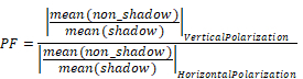(1):

(1)

From Table 2 it can be deduced that the larger the enclosure is, the greater the differences found between non-shadowed and shadowed data for vertical polarization. The results of this study show a more significant underestimation in vertical than in horizontal polarization, because for frequencies around 2,100 MHz, the localized SAR in limbs and head/trunk is higher for vertical polarization, in a standing position, and when waves impinge on the body from the front or back¹⁷. In addition, the user is not small in comparison to the wavelength, so the vertical polarization is at a worst-case level in terms of absorption of the incident wave²⁴. When the major axis of the human body is parallel to the electric field vector (which happens when the polarization of the biconical antenna is vertical), the specific absorption rate (SAR) of the human body reaches maximum values¹⁹. Theoretically, the vertically polarized waves are largely shielded by the human body, in comparison to the horizontally polarized waves. This is due to the fact that in vertical polarization, the E-field oscillates parallel to the long axis of the wearer⁸. As the polarization of the antenna is a key factor in the BSE, the proper polarization is vertical, in order to detect the maximum influence of the presence of the user on the measurements of the worn PEM and in NLoS²⁰.

The exposure levels obtained in the four enclosures under test conditions are shown in Figure 7 in a semi-logarithmic scale. The simulation results are shown together with the measurements at each point of the predefined route, demonstrating that both types of data vary in the same way in relation to their distance from the radiation source.

Table 3 summarizes the measured and simulated E-field levels, respectively. For each indoor enclosure the mean, standard deviation, and the maximum and minimum values are provided. It is worth noting the similarity between the statistical values of the experimental and simulated data. The similarity between each pair of experimental and simulated data series has also been checked in terms of the p-value obtained with the Kolmogorov-Smirnov (KS) test. The p-values are shown in Table 3. The p-values were always greater than the significance level of 0.05, so there is an adequate match between each pair of experimental and simulated data series. In addition, it has also been confirmed using the KS test that the cumulative distribution function (CDF) of each series, experimental or simulated, always follows the lognormal statistical distribution in both polarizations.

Figure 7 shows the measured and simulated data in the indoor enclosures being used for testing and the compliance with the thresholds established in the European legislation based on the ICNIRP, which forms the basis of many exposure standards presently applied worldwide in general, domestic, and occupational contexts. In the case of the general population, the limit of exposure to non-ionizing radiation at the 2.4 GHz frequency is 61 V/m. The value of 61 V/m established in the ICNIRP is not the most restrictive limit in terms of human exposure. Other standards exist around the world: in North America, IEEE establishes less restrictive limits: 66.7 V/m for uncontrolled environments, the equivalent for the general public in the ICNIRP. In addition, more restrictive regulation exists in Eastern Europe, such as the case of Russia where the strictest limit for the general population is 3.14 V/m. In Figure 7, the measurements compared with the ICNIRP threshold are not affected by the uncertainties of the PEM, providing reliability in the extracted conclusions with regard to regulation compliance.

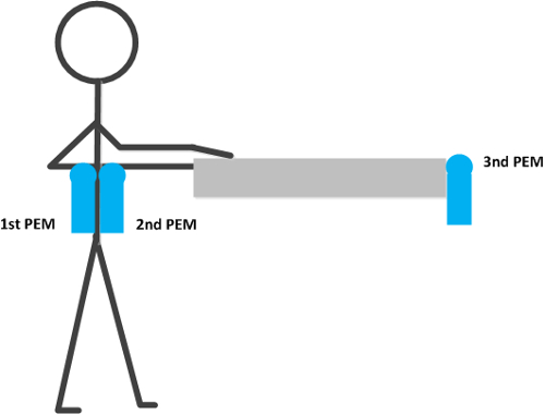
Figure 1: Location of the PEMs during the experiment.

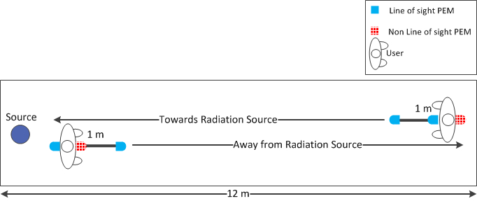
Figure 2: Predefined paths of control tests, towards and away from the radiation source, and position of the three dosimeters.

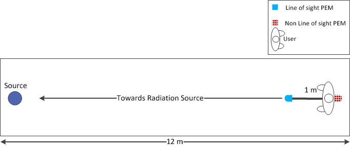
Figure 3: Predefined path of the measurement performed in the four enclosures, towards the radiation source, and positions of the dosimeters. The length of the test area within the first and second enclosures, 12 m, is shown.

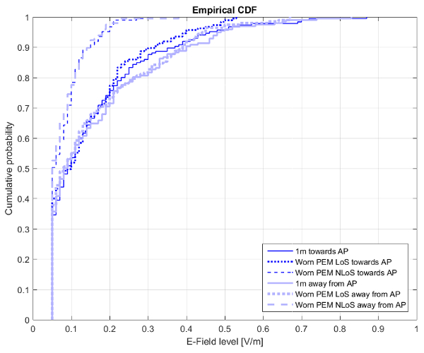
Figure 4: CDFs of the results of the three PEMs in different positions. Results are shown 1 m away, worn by the user in LoS, and worn by the user in NLoS for both predefined paths-towards and away from the radiation source.

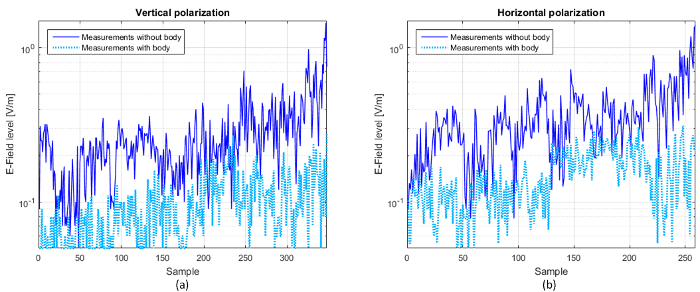
Figure 5: Experimental data obtained in the 63 m³ first enclosure. Data are shown for (a) vertical and (b) horizontal polarization, with and without body influence, with a transmission power of 100 mW. The data are shown in function of the number of samples logged by the PEM while the user is walking towards the source. The results are shown in a semi-logarithmic scale.

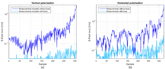
Figure 6: Experimental data obtained in the 162 m³ second enclosure. Data are shown for (a) vertical and (b) horizontal polarization, with and without body influence, with a transmission power of 25 dBm (316.12 mW) and rescaled to 20 dBm (100 mW). The data are shown as a function of the number of samples logged by the PEM while the user is walking towards the source. The results are shown in a semi-logarithmic scale.

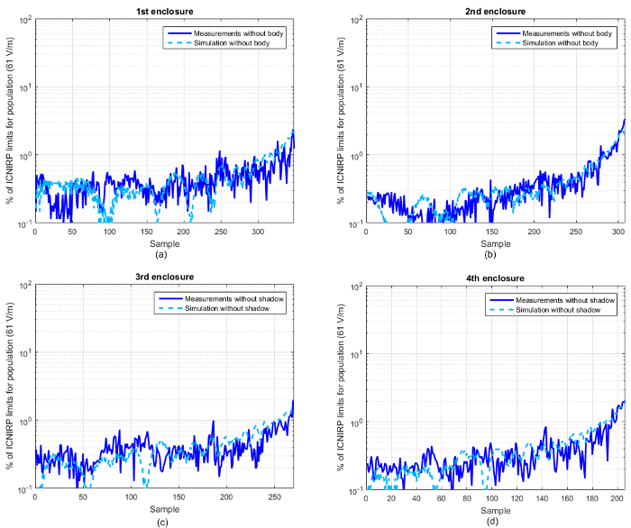
Figure 7: Measured and simulated levels of the E-field for vertical polarization. Levels are shown for the (a) first (63 m³), (b) second (162 m³), (c) third (57 m³), and (d) fourth (63 m³) enclosures. The levels are shown as a function of the percentage of the ICNIRP exposure limit of 61 V/m for the general population and for the 2.4 GHz band. The data are shown as a function of the number of samples logged by the PEM while the user is walking towards the source.

Material	Conductivity	Relative
	(S/m)	permittivity
Ceiling – chipboard	0.001	2.5
Floor – Marble	0.00022	7
Lateral walls	0.005	3
Metal	100	3
Glass	1E-10	6
Wood	0.0006	2

Table 1: Electromagnetic parameters used in the simulation.

Enclosure	Volume	Polarization
	(m3)	Factor
1	63	1.0635
2	162	1.3325
3	57	1.0235
4	63	1.0590

Table 2: Polarization factor for each enclosure, calculated as the relation between the means of non-shadow and shadow data. The sizes of the enclosures are indicated.

Enclosure	Size	Mean (V/m)		Std (V/m)		Max (V/m)		Min (V/m)		p-value	p-value
	(m3)	Exp	Sim	Exp	Sim	Exp	Sim	Exp	Sim	PolV	PolH
1	63	0.27	0.29	0.17	0.22	1.45	1.36	0.05	0.05	0.7296	0.8924
2	162	0.22	0.24	0.2	0.23	1.47	1.41	0.05	0.05	0.4579	0.3802
3	57	0.25	0.26	0.15	0.17	1.18	0.9	0.05	0.05	0.3740	0.3452
4	63	0.23	0.25	0.20	0.21	1.24	1.18	0.05	0.05	0.4679	0.4263

Table 3: Main statistical values of the experimental and simulated results in the four enclosures under test conditions for vertical and horizontal polarization. The sizes of the enclosures are indicated.

Discussion

The aspect of this protocol that is essential for the reliable collection of exposure data, without the influence of the PEM uncertainties, is the location of the PEM. The PEM must be situated 1 m away from the user in order to avoid underestimation caused by the influence of the body, and implicitly, to avoid a high number of non-detects in the logged data. There are aspects of the protocol that can be altered; modifications and limitations of the proposed technique are assessed as follows.

The measurement instrument selected to carry out the experiment is the PEM, which has been used in numerous studies for the analysis of EMF exposure in outdoor environments, dynamically, and in large geographical areas^24,25,26. Although data measured with the PEMs are not as accurate as the measurements provided by a spectrum analyzer (SA), numerous epidemiological studies use PEMs due to their easy handling and measuring rate²⁶, 4 s being the minimum sampling period. The PEMs used in the work have a minimum limit of sensitivity range of 0.05 V/m. More modern PEMs have been marketed with wider sensitivity ranges, 0.005 V/m being the lowest limit for the frequency band of 2.4 GHz, so the number of non-detects will be lower when the body is shielding the PEM. However, this fact is not relevant for this experiment, since the obtained results without the BSE uncertainty were always greater than 0.05 V/m. There are other models of PEMs with lower sampling periods, but the model used in this experiment has been selected because it is easily portable on the body, at waist height, where the body is maximally shielding the PEM.

In preliminary experiments, a Wi-Fi AP operating at the Wi-Fi frequency band of 2.4 GHz was employed as a radiation source. After assessing the power emitted by the AP with a SA, a check was carried out to confirm that the information packets were not transmitted continuously and that there were periods of time without transmission^27,28. As a consequence, a substantial proportion of RF EMF levels were below the detection limit (0.05 V/m) of the PEMs. The minimum Wi-Fi AP duty cycle was fixed by beacon signals and was around 0.01%. Meanwhile, a continuous signal, with the upper duty cycle limit of 100%, reproduces the worst-case exposure conditions, while avoiding the non-detects uncertainty. For this reason, a signal generator and a biconical antenna were used as radiation sources to generate a continuous wave of 100 mW power, at the Wi-Fi frequency, and without modulation.

The E-field levels, in the four selected indoor enclosures, have been predicted with a ray-tracing software based on image theory. The evaluation of the experimental results using another experimental technique, such as a SA with a probe, has not been considered, since the objective is to analyze the influence of the BSE and other PEM uncertainties, and not the PEM's ability to operate as another measuring device. The limitations of image theory are due to the non-ideal environmental conditions, that is, when the reflecting surfaces are not thin, flat, or planar. The propagation model results collect the uncertainty of reflection coefficients when the environmental conditions are non-ideal. When the surfaces are limited in extent, it is possible to eliminate the rays that do not intercept with them. As the number of reflections increases, the size of the Fresnel ellipsoids increases, and the approximation is worse. However, the rays from multiple reflections will be weaker and have less influence on the final results.

The naïve approach is applied to solve the uncertainty of the non-detects. This method consists of the substitution of the values below the sensitivity range limit with the lower detection limit²⁹. Other methods exist to correct the uncertainty of non-detects with the substitution of logged data. The robust regression on order statistics (ROS) method predicts the undetected values, considering that they follow a lognormal distribution. Other methods can be applied to the data, but the estimates always present a margin of error. The method of substitution by the lower detection limit has been used, as the substitution by a fixed value allows the identification of the non-detects. Additionally, this region of the CDFs does not present relevant differences among the several cases under analysis.

The uncertainty of the shadow effect of the human body must be addressed with special interest, given that PEMs are designed to be worn by the user, and the presence of the wearer is the cause of this uncertainty. In addition, the underestimation of the BSE may involve an increase in non-detects. The BSE can also be avoided by wearing several PEMs on different parts of the body^30,31; averaging the logged data of two PEMs situated on opposite sides of the body leads to a smaller underestimation, and a smaller uncertainty than the logged data of one single PEM⁵. Another alternative method is to take into account the alteration of the exposure levels due to the BSE in the interpretation of the exposure data and to apply appropriate correction factors. However, these have to be determined individually in function of the activity and the environment, and are very complex to apply correctly. Also, the technique used in this study proposes a practical way to avoid the BSE that only requires a single PEM, avoiding the processing of data.

Taking into account the advances in mobile technology, and the interest in the human body attenuation in future 5G (fifth generation) radio systems³², the technique presented in this study can be used to evaluate human exposure to new generation networks avoiding the aforementioned uncertainties.

Materials

List of materials used in this article

Name	Company	Catalog Number	Comments
Personal exposimeter	SATIMO	EME SPY 121/100	Worn personal exposimer to log expsure data
Personal exposimeter	ANTENNESSA	EME SPY 121/120	Worn personal exposimer to log expsure data
Wi-Fi Access Point	CISCO	Aironet 1130	Wi-Fi access point, vertial polarization
Analog Signal Generator	AGILENT	N5181A MXG	Analog Signal Generator
Precision Conical Dipole	SEIBERSDORF	PCD 8250	Broadband antenna 80 MHz - 3 GHz. Dipole-like radiation pattern that is omnidirectional in the horizontal plane
Cable	ROHDE & SCHWARZ	LARG-214/U	Low loss cable

References

- Aguirre, E., et al. Analysis of estimation of electromagnetic dosimetric values from non-ionizing radiofrequency fields in conventional road vehicle environments. Electromagn. Biol. and Med. 34 (1), 19-28 (2015).
- Aguirre, E., et al. Estimation of electromagnetic dosimetric values from non-ionizing radiofrequency fields in an indoor commercial airplane environment. Electromagn. Biol. and Med. 33 (4), 252-263 (2014).
- Barbiroli, M., Carciofi, C., Guiducci, D. Assessment of population and occupational exposure to Wi-Fi systems: Measurements and simulations. IEEE Trans. Electromagn. Compat. 53 (1), 219-228 (2011).
- Knafl, U., Lehmann, H., Riederer, M. Electromagnetic field measurements using personal exposimeters. Bioelectromagnetics. 29 (2), 160-162 (2008).
- Bolte, J. F. Lessons learnt on biases and uncertainties in personal exposure measurement surveys of radiofrequency electromagnetic fields with exposimeters. Environ. Int. 94, 724-735 (2016).
- Bechet, P., Miclaus, S., Bechet, A. C. Improving the accuracy of exposure assessment to stochastic-like radiofrequency signals. IEEE Trans. Electromag. Comp. 54 (5), 1169-1177 (2012).
- Najera Lopez, A., Gonzalez-Rubio, J., Villalba Montoya, J. M., Arribas, E. Using multiple exposimeters to evaluate the influence of the body when measuring personal exposition to radio frequency electromagnetic fields. COMPEL. 34 (4), 1063-1069 (2015).
- Bolte, J. F. B., van der Zande, G., Kamer, J. Calibration and uncertainties in personal exposure measurements of radiofrequency electromagnetic fields. Bioelectromagnetics. 32 (8), (2011).
- Blas, J., Lago, F. A., Fernández, P., Lorenzo, R. M., Abril, E. J. Potential exposure assessment errors associated with bodyworn RF dosimeters. Bioelectromagnetics. 28 (7), 573-576 (2007).
- Rodríguez, B., Blas, J., Lorenzo, R. M., Fernández, P., Abril, E. J. Statistical perturbations in personal exposure meters caused by the human body in dynamic outdoor environments. Bioelectromagnetics. 32 (3), 209-217 (2011).
- De Miguel-Bilbao, S., García, J., Ramos, V., Blas, J. Assessment of human body influence on exposure measurements of electric field in indoor enclosures. Bioelectromagnetics. 36 (2), 118-132 (2015).
- Neubauer, G., et al. The association between exposure determined by radiofrequency personal exposimeters and human exposure: A simulation study. Bioelectromagnetics. 31 (7), 535-545 (2010).
- Ghaddar, M., Talbi, L., Denidni, T. A., Sebak, A. A conducting cylinder for modeling human body presence in indoor propagation channel. IEEE Trans. Antennas Propag. 55 (11), 3099-3103 (2007).
- Thielens, A., et al. Personal distributed exposimeter for radio frequency exposure assessment in real environments. Bioelectromagnetics. 34 (7), 563-567 (2013).
- De Miguel-Bilbao, S., et al. Analysis of exposure to electromagnetic fields in a healthcare environment: Simulation and experimental study. Health Phys. 105 (5), S209-S222 (2013).
- Catedra, M. F., et al. Efficient ray-tracing techniques for three-dimensional analyses of propagation in mobile communications: application to picocell and microcell scenarios. IEEE Antennas Propagat. Mag. 40 (2), 15-28 (1998).
- Uusitupa, T., Laakso, I., Ilvonen, S., Nikoskinen, K. SAR variation study from 300 to 5000 MHz for 15 voxel models including different postures. Phys. Med. Biol. 55 (4), 1157-1176 (2010).
- Helsel, D. R. Fabricating data: How substituting values for nondetects can ruin results and what can be done about it. Chemosphere. 65 (11), 2434-2439 (2006).
- Ahlbom, A., et al. Guidelines for limiting exposure to time-varying electric, magnetic, and electromagnetic fields (up to 300 GHz). Health Phys. 74 (4), 494-522 (1998).
- De Miguel-Bilbao, S., Ramos, V., Blas, J. Assessment of polarization dependence of body shadow effect on dosimetry measurements in 2.4 GHz band. Bioelectromagnetics. 38 (4), 315-321 (2017).
- Lopez-Iturri, P., De Miguel-Bilbao, S., Aguirre, E., Azpilicueta, L., Falcone, F., Ramos, V. Estimation of radiofrequency power leakage from microwave ovens for dosimetric assessment at nonionizing radiation exposure levels. Biomed. Res. Int. 603260, 1-14 (2015).
- De Miguel-Bilbao, S., et al. Evaluation of electromagnetic interference and exposure assessment from s-health solutions based on Wi-Fi devices. Biomed. Res. Int. 784362, 1-9 (2015).
- Vermeeren, G., Joseph, W., Martens, L. Whole-body SAR in spheroidal adult and child phantoms in realistic exposure environment. Electron. Lett. 44 (13), 1-2 (2008).
- Beekhuizen, J., Vermeulen, R., Kromhout, H., Bürgi, A., Huss, A. Geospatial modelling of electromagnetic fields from mobilephone base stations. Sci. Total Environ. 445, 202-209 (2013).
- Gonzalez-Rubio, J., Najera, A., Arribas, E. Comprehensive personal RF-EMF exposure map and its potential use in epidemiological studies. Environ. Res. 149, 105-112 (2016).
- Urbinello, D., Huss, A., Beekhuizen, J., Vermeulen, R., Röösli, M. Use of portable exposure meters for comparing mobile phone base station radiation in different types of areas in the cities of Basel and Amsterdamn. Sci. Total Environ. 468, 1028-1033 (2014).
- Fang, M., Malone, D. Experimental verification of a radiofrequency power model for Wi-Fi technology. Health Phys. 98 (4), 574-583 (2010).
- Miclaus, S., Bechet, P. Electromagnetic field strength in proximity of WLAN devices during data and video file transmission. Electron. Lett. 50 (19), 1397-1399 (2014).
- Röösli, M., et al. Statistical analysis of personal radiofrequency electromagnetic field measurements with nondetects. Bioelectromagnetics. 29 (6), 471-478 (2008).
- Thielens, A., et al. On-body calibration and measurements using a personal, distributed exposimeter for wireless fidelity. Health Phys. 108 (4), 407-418 (2015).
- Thielens, A., et al. On-body calibration and processing for a combination of two radio frequency personal exposimeters. Radiat. Prot. Dosim. 163 (1), 58-69 (2015).
- Zhao, X., et al. Attenuation by human bodies at 26-and 39.5-GHz millimeter wavebands. IEEE Antennas Wireless Propag. Lett. 16, 1229-1232 (2017).
Reprints and Permissions