Transcription Start Site Mapping Using Super-low Input Carrier-CAGE

Summary

Cap Analysis of Gene Expression (CAGE) is a method for genome-wide quantitative mapping of mRNA 5’ends to capture RNA polymerase II transcription start sites at a single-nucleotide resolution. This work describes a low-input (SLIC-CAGE) protocol for generation of high-quality libraries using nanogram-amounts of total RNA.

Abstract

Cap analysis of gene expression (CAGE) is a method used for single-nucleotide resolution detection of RNA polymerase II transcription start sites (TSSs). Accurate detection of TSSs enhances identification and discovery of core promoters. In addition, active enhancers can be detected through signatures of bidirectional transcription initiation. Described here is a protocol for performing super-low input carrier-CAGE (SLIC-CAGE). This SLIC adaptation of the CAGE protocol minimizes RNA losses by artificially increasing the RNA amount through use of an in vitro transcribed RNA carrier mix that is added to the sample of interest, thus enabling library preparation from nanogram-amounts of total RNA (i.e., thousands of cells). The carrier mimics the expected DNA library fragment length distribution, thereby eliminating biases that could be caused by the abundance of a homogenous carrier. In the last stages of the protocol, the carrier is removed through degradation with homing endonucleases and the target library is amplified. The target sample library is protected from degradation, as the homing endonuclease recognition sites are long (between 18 and 27 bp), making the probability of their existence in the eukaryotic genomes very low. The end result is a DNA library ready for next-generation sequencing. All steps in the protocol, up to sequencing, can be completed within 6 days. The carrier preparation requires a full working day; however, it can be prepared in large quantities and kept frozen at -80 °C. Once sequenced, the reads can be processed to obtain genome-wide single-nucleotide resolution TSSs. TSSs can be used for core promoter or enhancer discovery, providing insight into gene regulation. Once aggregated to promoters, the data can also be used for 5’-centric expression profiling.

Introduction

Cap analysis of gene expression (CAGE) is a method used for single-nucleotide resolution genome-wide mapping of RNA polymerase II transcription start sites (TSSs)¹. Its quantitative nature also allows 5’-end centric expression profiling. Regions surrounding the TSSs (about 40 bp upstream and downstream) are core promoters and represent the physical location where RNA polymerase II and general transcription factors bind (reviewed previously^2,3). Information on exact locations of TSSs can be used for core promoter discovery and for monitoring promoter dynamics. In addition, as active enhancers exhibit signatures of bidirectional transcription, CAGE data can also be used for enhancer discovery and monitoring of enhancer dynamics⁴. CAGE methodology has recently increased in popularity due to its broad application and use in high-profile research projects such as ENCODE⁵, modENCODE⁶, and FANTOM projects⁷. In addition, TSS information is also proving to be important for distinguishing healthy and diseased tissue, as disease-specific TSSs can be used for diagnostic purposes⁸.

Even though several methods for TSS mapping are available (CAGE, RAMPAGE, STRT, nanoCAGE, nanoCAGE-XL, oligo-capping), we and others have recently shown that CAGE is the most unbiased method to capture true TSSs with the least number of false positives^9,10. The recent CAGE protocol, nAnT-iCAGE¹¹, is the most unbiased protocol for TSS profiling, as it avoids cutting the fragments to short tags using restriction enzymes and does not use PCR amplification. A limitation of the nAnT-iCAGE protocol is the requirement for a large amount of starting material (e.g., 5 µg of total RNA for each sample). To answer specific, biologically relevant questions, it is often impossible to obtain such high amounts of starting material (e.g., for FACS-sorted cells or early embryonic stages). Finally, if nAnT-iCAGE is successful, only 1-2 ng of DNA library material is available from each sample, thereby limiting the achievable sequencing depth.

To enable TSS profiling using only nanograms of total RNA, we have recently developed Super-low Input Carrier-CAGE¹⁰ (SLIC-CAGE, Figure 1). SLIC-CAGE requires only 10 ng of total RNA to obtain high complexity libraries. Our protocol relies on the carefully designed synthetic RNA carrier added to the RNA of interest to achieve a total of 5 μg of RNA material. The synthetic carrier mimics the target DNA library in length distribution to avoid potential biases that could be caused by homogenous molecules in excess. The sequence of the carrier is based on the sequence of the Escherichia coli leucyl-tRNA synthetase gene (Table 1) for two reasons. First, any leftover of the carrier in the final library, even if sequenced, will not map to a eukaryotic genome. Second, as E. coli is a mesophilic species, its housekeeping genes are optimised for the temperature range appropriate for SLIC-CAGE. The carrier sequence is also embedded with homing endonuclease recognition sites to allow specific degradation of DNA derived from the carrier RNA molecules. The target, sample-derived library remains intact, as the homing endonuclease recognition sites are long (I-CeuI = 27 bp; I-SceI = 18 bp) and statistically unlikely to be found in eukaryotic genomes. After specific degradation of the carrier and removal of fragments by size exclusion, the target library is PCR amplified and ready for next-generation sequencing. Depending on the starting RNA amount (1-100 ng), between 13-18 PCR amplification cycles are expected to be required. The final amount of DNA per each sample ranges between 5-50 ng, yielding enough material for very deep sequencing. When using only 1-2 ng of total RNA, true TSSs can be detected; however, the libraries are expected to be of lower complexity. Lastly, as SLIC-CAGE is based on the nAnT-iCAGE protocol¹¹, it enables multiplexing of up to eight samples prior to sequencing.

Protocol

1. Preparation of the Carrier

1. Preparation of DNA templates for in vitro transcription
   1. Prepare the PCR mix for each PCR template by combining 41 µL of water, 20 µL of 5x HF buffer, 8 µL of 2.5 mM dNTPs, 10 µL of 10 µM unique forward primer (PCR_GN5_f1, Table 2; primers are dissolved and diluted in water), 10 µL of 2 ng/µL template plasmid containing the synthetic carrier gene and 1 µL Phusion polymerase. Mix the PCR mix by pipetting. A master mix for all 10 templates can be prepared at once (prepare for 11 reactions).
   2. Add 90 µL of the PCR mix to 10 µL of each 10 µM reverse primer (PCR_N6_r1-r10, Table 2). Mix by pipetting.
   3. PCR amplify the templates using the following program: 98 °C for 60 s, (98 °C for 10 s, 50 °C for 30 s, 72 °C for 30 s) 35 cycles, 72 °C for 10 min, hold at 4 °C.
   4. Gel purification of PCR-amplified DNA templates
      1. Prepare a 1% agarose gel (low-melting agarose is recommended).
      2. To decrease the volume, concentrate the PCR reaction mixtures from 100 µL to 20 µL total volume using the vacuum concentrator at a low-medium temperature (30–40 °C).
      3. Add 6 µL of the 6x loading dye, mix well, and load on the gel. Run electrophoresis for 30 min in 1x TAE buffer at the voltage appropriate for the used electrophoresis tank (5–10 V/cm). In parallel run a 100 bp or 1,000 bp DNA ladder.
      4. Using a clean scalpel, excise the gel slices containing the target PCR product. Avoid excess agarose gel. Purify the PCR products using a gel extraction kit (according to the manufacturer’s instructions).
         NOTE: A260/A230 ratios of DNA isolated from agarose gels are typically low (0.1–0.3). Expected target product and side products are shown in Figure 2A. Expected yields from 100 µL PCR reactions are 1.2–3 µg. Reactions can be scaled up to get a higher yield.
2. In vitro transcription of carrier molecules
   1. Transcribe carrier RNA in vitro using the T7 RNA polymerase according to the manufacturer’s instructions. Set up 10–20 µL reactions (the recommended kit is in Table of Materials).
   2. Purify the in vitro transcribed RNA using an RNA purification kit. Set up DNA digestion in solution using DNase I following the manufacturer’s standard instructions, and elute the RNA in 50 µL of water. To increase the elution yield, leave the water in the column for 5 min before centrifugation.
      NOTE: Be careful not to exceed the maximum binding capacity of the columns (in the kit mentioned in the Table of Materials, capacity is up to 100 µg). The expected yield from PCR templates 1–10 (1 kbp to 200 bp in length) is 25–50 µg from 10 µL in vitro transcription reactions. Reactions can be scaled up to get a larger stock of carrier molecules.
3. Capping of in vitro transcribed carrier RNA molecules
   1. Prepare the capping mix by combining 2 µL of 10x capping buffer, 1 µL of 10 mM GTP, 1 µL of 2 mM SAM (freshly diluted) ,and 1 µL of Vaccinia capping enzyme per carrier RNA.
   2. Mix up to 10 µg of each carrier molecule in 15 µL of total volume and denature for 10 min at 65 °C. Place on ice immediately to prevent secondary structure formation.
   3. Mix the denatured carrier RNA with 5 µL of the capping mix and incubate for 1 h at 37 °C.
   4. Purify capped RNA molecules using an RNA purification kit — follow the manufacturer’s clean-up protocol. Elute RNA in 30 µL of water. To increase the elution yield, leave the water in the column for 5 min before centrifugation.
      NOTE: Measure concentration using the microvolume spectrophotometer. Expected A260/A280 ratio is >2 and A260/A230 is >2. Note that for some RNA samples A260/A230 may be between 1.3–2. Expected yield when using 10 µg of uncapped RNA is 9–10 µg of capped RNA.
4. Prepare the mix of the capped and uncapped carrier by combining the amounts described in Table 3. Mix well by flicking the tube and measure the concentration using the microvolume spectrophotometer.
   NOTE: If a higher concentration of the carrier is required to fit in the reverse transcription reaction (see below), the carrier mix can be concentrated using the vacuum concentrator at low-medium temperature (30-35 °C) until reaching the desired final concentration. Steps 2–14 are modified from the standard nAnT-iCAGE protocol reported by Murata et al.¹¹

2. Reverse Transcription

1. Combine 1 µL of the RT primer (2.5 mM TCT-N6 dissolved in water, for sequence see Supplementary Table 1), 10 ng of total RNA of interest and 4,990 ng of carrier mix (Table 3) in 10 µL of total volume in a low-binding PCR plate. Mix by flicking the tube.
   NOTE: If the sample RNA is too diluted for reverse transcription (see below), combine it with the appropriate amount of the carrier, concentrate using the vacuum concentrator to 9 µL total volume, and add 1 µL of the RT primer. Adding the carrier earl, to reach 5 µg of RNA in total prevents sample loss.
2. Heat the mix from step 2.1 at 65 °C for 5 min, and place on ice immediately to prevent renaturation.
3. Prepare of the reverse transcription (RT) mix.
   1. For each sample combine 6.1 µL of water (RNase- and DNase-free), 7.6 µL of 5x first-strand buffer, 1.9 µL of 0.1 M DTT, 1 µL of 10 mM dNTPs, 7.6 µL of trehalose/sorbitol mix (see recipe in Murata et al.¹¹) and 3.8 µL of the recommended reverse transcriptase (see Table of Materials). Mix well by flicking the tube.
4. Add 28 µL of the RT mix into the PCR tube with 10 µL of RNA, carrier and the RT primer (total volume 38 µL). Mix well by pipetting.
   NOTE: The mix is highly viscous due to trehalose/sorbitol. Mix until visibly homogenous.
5. Incubate in a thermal cycler using the following program: 25 °C for 30 s, 50 °C for 60 min, and hold at 4 °C.
6. Purification of cDNA:RNA hybrids using SPRI magnetic beads
   1. Add 68.4 µL of the recommended RNAse- and DNase-free SPRI beads (see Table of Materials) to 38 µL of the RT mix (beads to sample ratio 1.8:1). Mix well by pipetting and incubate for 5 min at room temperature (RT).
   2. Separate the beads on a magnetic stand for 5 min. Discard the supernatant and wash the beads twice with 200 µL of 70% ethanol (freshly prepared).
      NOTE: The ethanol is added to the beads without mixing and while the tube is on the magnetic stand. The added ethanol is immediately removed. Care should be taken not to lose any beads during washes as it may lead to sample loss.
   3. While the tube is still on the magnetic stand, remove all traces of ethanol. Droplets of ethanol can be removed and pushed out of the tube using a P10 pipette. Do not let the beads dry.
   4. Add 42 µL of water preheated at 37 °C to the beads and elute the sample by pipetting up and down 60x.
      NOTE: Be careful not to cause foaming by pipetting as it may cause loss of beads (i.e., bound sample) in the foam.
   5. Incubate at 37 °C for 5 min without the lid to allow evaporation of trace amounts of ethanol.
   6. Separate the beads on a magnetic stand for 5 min and transfer the supernatant to a new plate.
      NOTE: Try to retrieve all the supernatant to prevent sample loss while avoiding bead carryover. Use the P10 pipette to get the last sample droplets.

3. Oxidation

1. Add 2 µL of 1 M NaOAc (pH 4.5) into the purified RT reaction. Mix by pipetting, add 2 µL of 250 mM NaIO₄ and mix again.
2. Incubate on ice for 45 min. Cover the plate with aluminum foil to avoid light.
3. Add 16 µL of Tris-HCl (pH 8.5) into the oxidation mix to neutralize the pH.
4. Purify oxidized cDNA:RNA hybrids using SPRI magnetic beads. Add 108 µL of SPRI beads to 60 µL of the oxidation mix (1.8:1 beads to sample ratio). Repeat the purification as described in steps 2.6.1–2.6.6. Elute using 42 µL of water preheated to 37 °C.
   NOTE: Freshly prepare 250 mM NaIO₄ by adding 18.7 µL of water per 1 mg of NaIO₄. NaIO₄ is light-sensitive; therefore, keep the solution in a tube covered with aluminum foil or in a light-resistant tube.

4. Biotinylation

1. Add 4 µL of 1 M NaOAc (pH 6.0) into the tube containing the purified oxidized sample and mix by pipetting.
2. Add 4 µL of 10 mM biotin solution, mix by pipetting and incubate for 2 h at 23 °C in a thermal cycler to avoid light.
   NOTE: Prepare the biotin solution by mixing 50 mg of biotin with 13.5 mL of DMSO. Make single-use aliquots and freeze at -80 °C.
3. Purify biotinylated cDNA:RNA hybrids using SPRI magnetic beads. Add 12 µL of 2-propanol and mix by pipetting. Add 108 µL of SPRI beads (1.8:1 beads to sample ratio) and repeat the purification as described in steps 2.6.1–2.6.6. Elute using 42 µL of water preheated at 37 °C.
   NOTE: The protocol can be paused here, and samples frozen at -80 °C.

5. RNase I Ddigestion

1. Prepare the RNase I mix by mixing 4.5 µL of 10x RNase I buffer with 0.5 µL of RNase I (10 U/µL) per each sample. Mix by pipetting.
2. Add 5 µL of the mix to each purified sample (45 µL in total). Mix by pipetting and incubate for 30 min at 37 °C.

6. Preparation of Streptavidin Beads

1. For each sample, mix 30 µL of the streptavidin beads slurry with 0.38 µL of 20 mg/mL tRNA. Incubate on ice for 30 min and mix every 5 min by flicking the tube.
   NOTE: Resuspend the streptavidin beads slurry well before pipetting by flicking the bottle. The tRNA solution should be prepared according to Murata et al.¹¹
2. Separate the beads on the magnetic stand for 2–3 min. Remove the supernatant.
3. Wash the beads by resuspending in 15 µL of buffer A. Separate the beads on the magnetic stand for 2–3 min and remove the supernatant. Repeat the wash and remove the supernatant.
4. Resuspend the beads in 105 µL of buffer A and add 0.19 µL of 20 mg/mL of tRNA. Mix well by pipetting.
   NOTE: The beads should be prepared fresh prior to use. Start preparation of the beads during RNase I digestion. For multiple samples prepare the beads together in a single tube.

7. Cap-trapping

1. Sample binding
   1. Add 105 µL of prepared streptavidin beads to 45 µL of the RNase I-treated sample. Mix well by pipetting and incubate at 37 °C for 30 min. Mix by pipetting every 10 min.
   2. Separate the beads on the magnetic stand for 2–3 min. Remove the supernatant.
2. Washing beads
   1. Add 150 µL of wash buffer A and resuspend the beads by pipetting. Separate the beads on the magnetic stand for 2–3 min and remove the supernatant.
   2. Add 150 µL of the wash buffer B and resuspend the beads by pipetting. Separate the beads on the magnetic stand for 2–3 min and remove the supernatant.
   3. Add 150 µL of the wash buffer C and resuspend the beads by pipetting. Separate the beads on the magnetic stand for 2–3 min and remove the supernatant.
      NOTE: Buffers B and C should be preheated to 37 °C. Recipes for wash buffers A, B, and C are as described in Murata et al.¹¹
3. cDNA release
   1. Prepare 1x RNase I buffer by mixing 58.5 µL of water with 6.5 µL of 10x RNase I buffer.
   2. Resuspend the beads in 35 µL of 1x RNase I buffer. Incubate at 95 °C for 5 min and transfer directly on ice for 2 min to prevent reassociation of cDNA. Hold the lids during transfer to ice as they may pop-off due to pressure build up.
   3. Separate the beads for 2–3 min on a magnetic stand and transfer the supernatant to a new plate.
   4. Resuspend the beads in 30 µL of 1x RNase I buffer. Separate the beads on the magnetic stand for 2–3 min and transfer the supernatant to the previously collected supernatant (total volume of eluted cDNA should be about 65 µL).

8. RNA Removal by RNase H and RNase I Digestion

1. Per sample, combine 2.4 µL of water, 0.5 µL of 10x RNase I buffer, 0.1 µL of RNase H, and 2 µL of RNase I.
2. Add 5 µL of the mix to the 65 µL of the released cDNA sample and mix by pipetting. Incubate at 37 °C for 15 min and hold at 4 °C.
3. Purify cDNA from the RNase digestion mix using SPRI magnetic beads. Add 126 µL of SPRI beads to 70 µL of degradation reaction and mix by pipetting. Follow purification steps as described for SPRI beads purification in 2.6.1–2.6.6. Elute using 42 µL of water preheated at 37 °C as described.
4. Prepare RNase I mix by combining 4.5 µL of 10x RNase I buffer and 0.5 µL of RNase I.
5. Add 5 µL of the RNase mix to the 40 µL of the purified cDNA sample. Mix by pipetting and incubate at 37 °C for 30 min. Hold at 4 °C.
6. Purify the sample using SPRI magnetic beads. Add 81 µL of SPRI beads to 45 µL of degradation reaction and mix by pipetting. Follow purification steps as described for SPRI beads purification in 2.6.1–2.6.6. Elute using 42 µL of water as described.

9. Ligation of 5’ Linker

1. Concentrate the purified cDNA sample to 4 µL using the vacuum concentrator. Keep the temperature at 30–35 °C. Test the volume using a pipette. If the sample has dried to completeness, dissolve by adding 4 µL of water.
   NOTE: It is better to avoid drying to completeness to prevent sample loss.
2. Incubate the concentrated sample at 95 °C for 5 min and immediately place on ice for 2 min to prevent renaturation. Hold the lids while transferring the tubes as the lids may pop-off due to pressure build-up.
3. Incubate 4 µL of the 2.5 µM 5’ linker at 55 °C for 5 min and immediately place on ice for 2 min to prevent renaturation.
4. Mix 4 µL of the 2.5 µM 5’ linker with 4 µL of the sample.
   NOTE: The 5’ linker should be prepared according to Supplementary Table 2, Supplementary Table 3, Supplementary Table 4, and Supplementary Table 5. Dilute the 10 µM 5’ linker to a 2.5 µM concentration using 100 mM NaCl prior to use.
5. Add 16 µL of the ligation premix (see Table of Materials) to the mixed 5’ linker and the sample and mix well by pipetting. Incubate at 16 °C for 16 h.
6. Purify the ligation mix using SPRI magnetic beads. Add 43.2 µL of SPRI beads and follow steps 2.6.1–2.6.6. Elute as described using 42 µL of water preheated at 37 °C.
7. Repeat the purification done in step 9.6 by adding 72 µL of SPRI beads to the transferred supernatant (1.8:1 beads to sample ratio).
   NOTE: 5’ linkers contain barcodes which allows pooling of up to eight samples prior to sequencing (eight trinucleotide barcodes are available, as described in Murata et al.¹¹ and Supplementary Table 1).

10. Ligation of 3’ Linker

1. Concentrate the purified sample to 4 µL using the vacuum concentrator as described in step 9.1.
2. Incubate the concentrated sample at 95 °C for 5 min and immediately place on ice for 2 min to prevent renaturation. Hold the lids while transferring the tubes as the lids may pop off due to pressure build-up.
3. Incubate 4 µL of the 2.5 µM 3’ linker at 65 °C for 5 min and immediately place on ice for 2 min to prevent renaturation.
4. Add 4 µL of the 2.5 µM 3’ linker to the 4 µL of the concentrated sample.
5. Add 16 µL of the ligation premix and mix well by pipetting. Incubate at 16 °C for 16 h.
6. Purify the ligation mix using SPRI magnetic beads. Add 43.2 µL of SPRI beads and follow steps 2.6.1–2.6.6. Elute as described using 42 µL of water preheated to 37 °C.
   NOTE: The 3’ linker should be prepared according to Supplementary Tables 6 and Supplementary Table 7. Dilute the 10 µM 3’ linker to a 2.5 µM concentration using 100 mM NaCl.

11. Dephosphorylation

1. Prepare the SAP mix by combining 4 µL of water, 5 µL of 10x SAP buffer, and 1 µL of SAP enzyme.
2. Add 10 µL of SAP mix to the purified ligated sample (total volume 50 µL) and incubate in the thermocycler using the following program: 37 °C for 30 min, 65 °C for 15 min, and hold at 4 °C.

12. Degradation of 3’ Linker Upper Strand Using Uracil Specific Excision Enzyme

1. Add 2 µL of uracil specific excision enzyme (see Table of Materials) to the dephosphorylated sample, mix by pipetting and incubate in the thermocycler using the following program: 37 °C for 30 min, 95 °C for 5 min, and immediately place on ice for 2 min to prevent reannealing of the fragmented upper strand.
2. Purify the reaction mixture by adding 93.6 µL of SPRI magnetic beads to the 52 µl mixture and mix well by pipetting. Repeat purification steps 2.6.1–2.6.6. Elute with 42 µL of water preheated at 37 °C as described.

13. Second Strand Synthesis

1. Prepare the second strand synthesis mix (volumes are expressed per sample) by combining 5 µL of 10x DNA polymerase reaction buffer, 2 µL of water, 1 µL of 10 mM dNTPs, 1 µL of 50 µM nAnT-iCAGE second strand primer (sequence is in Supplementary Table 1) and 1 µL of DNA exonuclease-deficient polymerase (see recommended polymerase in Table of Materials).
2. Add 10 µL of the mix to the purified sample and mix well by pipetting (total volume is 50 µL). Incubate in the thermal cycler using the following program: 95 °C for 5 min, 55 °C for 5 min, 72 °C for 30 min, and hold at 4 °C.

14. Degradation of Second Strand Synthesis Primer Using Exonuclease I

1. Add 1 µL of Exonuclease I to the second strand synthesis mixture. Mix well by pipetting and incubate at 37 °C for 30 min followed by holding at 4 °C.
2. Purify double stranded DNA by adding 91.8 µL of SPRI magnetic beads to 51 µL of the Exonuclease I-treated sample. Repeat purification steps described in 2.6.1–2.6.6. and elute with 42 µL of water preheated to 37 °C as described.
3. Concentrate the sample using the vacuum concentrator to 15 µL as described in step 9.1.

15. Quality and Quantity Control

1. Use 1 µL of the concentrated samples and run a high sensitivity DNA chip on a DNA quality analyzer. Expected profile/quantity is presented in Figure 3.

16. First Round of Carrier Degradation

1. Prepare the degradation mix by combining 2 µL of water, 2 µL of 10x restriction enzyme buffer, 1 µL of I-SceI, and 1 µL of I-CeuI.
2. Add 6 µL of the degradation mix to 14 µL of the concentrated sample and mix by pipetting. Incubate at 37 °C for 3 h followed by 20 min deactivation at 65 °C and hold at 4 °C.
3. Purify the degradation mix using SPRI magnetic beads. Add 5 µL of water to increase the volume of the degradation mix and add 45 µL of SPRI beads (1.8:1 beads to sample ratio). Repeat purification as described in steps 2.6.1–2.6.6. and elute with 42 µL of water preheated to 37 °C.
4. Concentrate the eluted sample from 42 µL to 20 µL of the total volume as described in step 9.1.

17. Control of Degradation Level and Determining the Number of PCR Amplification Cycles

1. Prepare qPCR mix for amplifying whole libraries (adaptor mix). Combine 3.8 µL of water, 5 µL of qPCR premix (2x), 0.1 µL of 10 µM adaptor_f1 primer (5’-AATGATACGGCGACCACCGA-3’), and 0.1 µL of 10 µM adaptor_r1 primer (5’-CAAGCAGAAGACGGCATACGA-3’) for each sample (see Table of Materials for recommended qPCR premix).
2. Combine 9 µL of qPCR adaptor mix with 1 µL of sample from step 16.4 and mix well by pipetting.
3. Prepare qPCR mix for amplifying DNA derived from the carrier (carrier mix). Combine 3.8 µL of water, 5 µL of qPCR premix (2x), 0.1 µl of 10 µM carrier_f1 primer (5’-GCGGCAGCGTTCGCTATAAC-3’), and 0.1 µL of 10 µM adaptor_r1 primer for each sample
4. Combine 9 µL of qPCR carrier mix with 1 µL of the sample from step 16.4 and mix well by pipetting.
5. Set qPCR program: 95 °C for 3 min (95 °C for 20 s, 60 °C for 20 s, 72 °C for 2 min) repeated 40x, followed by instrument-specific denaturation curve (65–95 °C), and hold at 4 °C.
   NOTE: Prepare a negative control by replacing the sample with water.

18. PCR Amplification of the Target Library

1. Prepare the PCR amplification mix by combining 6 µL of water, 0.5 µL of 10 µM adaptor_f1 primer, 0.5 µL of 10 µM adaptor_r1 primer and 25 µL of PCR premix (2x). Mix by pipetting (see Table of Materials for the recommended PCR premix).
2. Add 32 µL of the PCR mix to 18 µL of the sample from step 16.4. Mix thoroughly by pipetting.
3. Set the PCR amplification: 95 °C for 3 min, (98 °C for 20 s, 60 °C for 15 s, 72 °C for 2 min) 12-18 cycles, 72 °C for 2 min and hold at 4 °C.
   NOTE: The exact number of PCR cycles is determined by qPCR results and corresponds to the Ct value obtained with the adaptor primer mix (number of PCR cycles is equal to the Ct value).
4. Purify the amplified sample by adding 90 µL of SPRI magnetic beads to 50 µL of the amplified sample and mix thoroughly by pipetting. Repeat the purification steps described in steps 2.6.1–2.6.6. and elute the sample using 42 µL of water as described.

19. Second Round of Carrier Degradation

1. Repeat steps 16.1–16.3.
2. Purify the degradation mix using SPRI magnetic beads. Add 10 µL of water to the sample to increase the volume and mix with 30 µL of SPRI beads (1:1 beads to sample ratio). Repeat purification as described in steps 2.6.1–2.6.6. and elute with 42 µL of water preheated at 37 °C as described.
3. Concentrate the eluted sample from 42 µL to 30 µL of total volume.

20. Library Size Selection

1. Mix 24 µL of SPRI magnetic beads with 30 µL of the sample from step 19.3. (0.8:1 beads to sample ratio). Repeat the purification steps as described in steps 2.6.1–2.6.6. and elute the sample in 42 µL of water as described.
2. Concentrate the sample to approximately 14 µL as described in step 9.1.

21. Quality Control

1. Assessment of size-distribution
   1. Run 1 µL of the sample on the high sensitivity DNA chip. Expected results are presented in Figure 4.
      NOTE: If fragments shorter than 200 bp are visible (see example in Figure 4A,C), size selection (steps 20.1–20.2) should be repeated until the short fragments are removed (Figure 4B,D). Usually one additional round of size selection is enough. If the amount of short fragments is severe (as in Figure 4C), the beads-to-sample ratio should be decreased to 0.6:1.
2. Carrier degradation quality control
   1. Repeat steps 17.1–17.5.
      NOTE: Depending on the concentration of the libraries estimated in the HS DNA chip run (region analysis), the samples need to be diluted prior to qPCR. Use 0.5 µL of the sample to avoid sample loss and dilute 100–500x in water (dilute to 1–20 pg/µL final concentration). Expected difference between Ct values obtained with adaptor and carrier mix is 5–10.
3. Library quantification
   1. Prepare the working dilution of the lambda DNA standard by mixing 20 µL of 100 mg/mL lambda DNA standard with 980 µL of 1x TE (prepare by diluting 20x TE provided in the DNA quantification kit). Dilution of the lambda DNA can be stored at -20 °C.
   2. Prepare the lambda DNA standard serial dilutions by mixing the diluted lambda standard and 1x TE according to Supplementary Table 8.
      NOTE: For higher accuracy, it is recommended to add 100 µL of 1x TE buffer to all tubes and remove 1x TE volume as required per volume of the diluted lambda to be added. Do not use more than 1 µL of the library; use of 384 well plates for this measurement is recommended.

Results

This report describes the full SLIC-CAGE protocol for obtaining sequencing-ready libraries from nanograms of starting total RNA material (Figure 1). To obtain the synthetic RNA carrier mix, first, PCR carrier templates need to be prepared and gel-purified to eliminate PCR side products (Figure 2A). Each PCR template (ten in total) is produced by using a common forward, but a different reverse primer (Table 2), leading to different lengths of the PCR template to enable size variability of synthetic RNA carriers. Once purified, PCR templates are used for in vitro transcription of the carrier molecules. A single RNA carrier product is expected if the templates are gel-purified (see representative gel-analysis in Figure 2B). Preparation of the carrier can be upscaled depending on the need, and when prepared, mixed and frozen at -80 °C for future use.

Using the recommended minimal amount of sample total RNA (10 ng) combined with 16-18 cycles of PCR amplification, high complexity SLIC-CAGE libraries can be achieved. Number of PCR cycles required to amplify the final library highly depends on the amount of total input RNA used (the expected number of cycles is presented in Table 4).

After the first round of degradation, in qPCR results (step 17), the expected difference between Ct values obtained using adaptor_f1 or carrier_f1 primer is 1-2, with Ct values obtained with adaptor_f1 lower than with carrier_f1.

The distribution of the fragment lengths in the final library is between 200-2,000 bp with the average fragment size of 700-900 bp (based on the region analysis using Bioanalyzer software, Figure 4B,D). Shorter fragments, as presented in Figure 4A,C, have to be removed by additional rounds of size-exclusion (steps 20-21). These short fragments are PCR amplification artefacts and not the target library. Note that shorter fragments cluster better on the sequencing flow cells and may cause sequencing problems.

The expected amount of library material obtained per sample is between 5-50 ng. Significantly lower amounts are indicative of sample loss during the protocol. If the obtained low quantity is enough for sequencing (2-3 ng of the pooled libraries is needed), the libraries may be of lower complexity (see below).

Depending on the sequencing machine, quantity of the library loaded onto the flow cell may need to be optimised. Using an Illumina HiSeq 2500, loading 8-12 pM SLIC-CAGE libraries gives on average 150-200 million reads, with >80% of reads passing quality score Q30 as threshold.

The obtained reads are then mapped to the reference genome [for 50 bp reads, Bowtie2¹² can be used with default parameters that allow zero mismatches per seed sequence (22 bp)]. Expected mapping efficiencies depend on the total RNA input amount and are presented in Table 5. The uniquely mapped reads can then be loaded into R graphical and statistical computing environment¹³ and processed using CAGEr (Bioconductor package¹⁴). The package vignette is easy to follow and explains the workflow and processing of the mapped data in detail. An easy visual control of the library complexity is the distribution of promoter width, as low-complexity libraries will have artificially narrow promoters (Figure 5A, SLIC-CAGE library derived from 1 ng of total RNA, for details see previous publication¹⁰). However, even the low-complexity SLIC-CAGE libraries allow identification of true CTSSs, with greater precision than alternative methods for low/medium-input TSS mapping (Figure 5B,C).

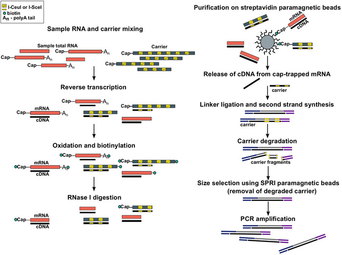
Figure 1: Steps in the SLIC-CAGE protocol. Sample RNA is mixed with the RNA carrier mix to achieve 5 µg of total RNA material. cDNA is synthesised through reverse transcription and the cap is oxidized using sodium periodate. Oxidation allows attachment of biotin to the cap using biotin hydrazide. Biotin gets attached to the mRNA’s 3′ end, as it is also oxidized using sodium periodate. To eliminate biotin from mRNA:cDNA hybrids with incompletely synthesized cDNA and from the 3′ ends of mRNA, the samples are treated with RNase I. cDNA that reached the 5′ end of mRNA is then selected by affinity purification on streptavidin magnetic beads (cap-trapping). After release of cDNA, 5′- and 3′-linkers are ligated. The library molecules that originate from the carrier are degraded using I-SceI and I-CeuI homing endonucleases and the fragments are removed using SPRI magnetic beads. The library is then PCR amplified. Please click here to view a larger version of this figure.

Figure 2: Representative gel-analysis of carrier PCR templates and carrier in vitro transcripts. (A) Carrier PCR templates prior to gel purification: the first well contains the 1 kbp marker, followed by carrier PCR templates 1, 1-10. (B) Carrier in vitro transcripts: the first well contains the 1 kbp marker, followed by carrier transcripts 1-10. Carrier transcripts were denatured by heating for 5 min at 95 °C prior to loading. Please click here to view a larger version of this figure.

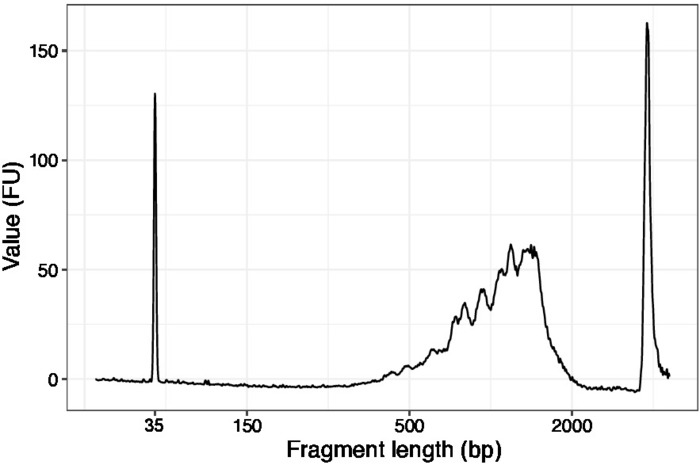
Figure 3: Representative DNA quality (high sensitivity DNA chip) trace of SLIC-CAGE prior to first round of carrier degradation. Please click here to view a larger version of this figure.

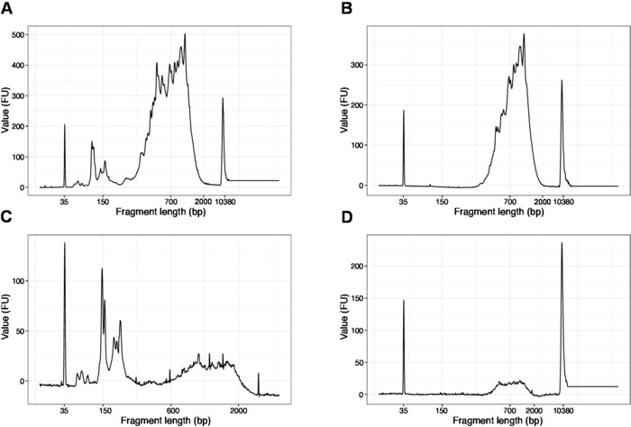
Figure 4: Representative DNA quality (high sensitivity DNA chip) traces of SLIC-CAGE libraries after PCR amplification. (A) SLIC-CAGE library that requires additional size-selection for removal of short fragments. (B) SLIC-CAGE library after size-selection using 0.6x SPRI beads to sample ratio. (C) SLIC-CAGE library of lower output amount that requires size-selection for removal of short fragment. (D) SLIC-CAGE library of lower output amount after size-selection using 0.6:1 SPRI beads to sample ratio. Please click here to view a larger version of this figure.

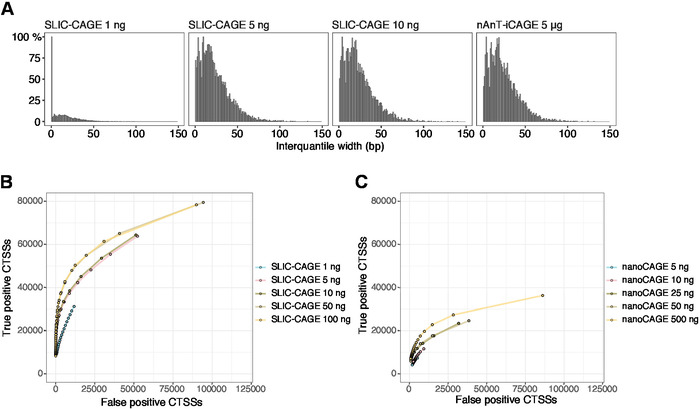
Figure 5: Validation of SLIC-CAGE libraries. (A) Distribution of tag cluster interquantile widths in SLIC-CAGE libraries prepared from 1, 5, or 10 ng of S. cerevisiae total RNA, and in the nAnT-iCAGE library prepared from 5 µg of S. cerevisiae total RNA. A high amount of narrow tag clusters in the 1 ng SLIC-CAGE library indicates its low complexity. (B) ROC curves for CTSS identification in S. cerevisiae SLIC-CAGE libraries. All S. cerevisiae nAnT-iCAGE CTSSs were used as a true set. (C) ROC curves for CTSS identification in S. cerevisiae nanoCAGE libraries. All S. cerevisiae nAnT-iCAGE CTSSs were used as a true set. Comparison of ROC curves shows that SLIC-CAGE strongly outperforms nanoCAGE in CTSS identification. Data from ArrayExpress E-MTAB-6519 was used. Please click here to view a larger version of this figure.

Table 1: Sequence of the carrier synthetic gene. I-SceI sites are bold and italicized in purple, and I-CeuI recognitions sites are green. Please click here to view this table (Right click to download).

carrier	reverse primer 5’-3’		PCR product length / bp
1	PCR_N6_r1: NNNNNNCTACGTGTCGCAGACGAATT		1034
2	PCR_N6_r2: NNNNNNTATCCAGATCGTTGAGCTGC		966
3	PCR_N6_r3: NNNNNNCACTGCGGGATCTCTTTACG		889
4	PCR_N6_r4: NNNNNNGCCGTCGATAACTTGTTCGT		821
5	PCR_N6_r5: NNNNNNAGTTGACCGCAGAAGTCTTC		744
6	PCR_N6_r6: NNNNNNGTGAAGAATTTCTGTTCCCA		676
7	PCR_N6_r7: NNNNNNCTCGCGGCTCCAGTCATAAC		599
8	PCR_N6_r8: NNNNNNTATACGCGATGTTGTCGTAC		531
9	PCR_N6_r9: NNNNNNACCGCCGCGCCTTCCGCAGG		454
10	PCR_N6_r10: NNNNNNCAGGACGTTTTTGCCCAGCA		386
	* Forward primer is the same for all carrier templates. Underlined is the T7 promoter sequence. PCR_GN5_f1: TAATACGACTCACTATAGNNNNNCAGCGTTCGCTA

Table 2: Primers for carrier template amplification. Forward primer is the same for all carrier templates. Underlined is the T7 promoter sequence. PCR_GN5_f1: TAATACGACTCACTATAGNNNNNCAGCGTTCGCTA. Using differing reverse primers, PCR templates and hence carrier RNAs of differing length are produced.

carrier	length	uncapped/µg	capped/µg
1	1034	3.96	0.45
2	966	8.36	0.95
3	889	4.4	0.5
4	821	6.6	0.75
5	744	4.4	0.5
6	676	3.08	0.35
7	599	4.4	0.5
8	531	3.96	0.45
9	454	2.64	0.3
10	386	2.2	0.25

Table 3: RNA carrier mix. In total 49 µg of the carrier mix 0.3-1 kbp: uncapped = 44 µg, capped = 5 µg.

Total RNA input /ng	PCR cycles
1 ng	18
2 ng	17
5 ng	16
10 ng	15-16
25 ng	14-15
50 ng	13-15
100 ng	12-14

Table 4: Expected number of PCR cycles in dependence of sample total RNA input. Approximate number of cycles is based on experiments performed using Saccharomyces cerevisiae, Drosophila melanogaster, and Mus musculus total RNA.

Total RNA input/ng	% overall mapped	% uniquely mapped	% carrier
1 ng	30	20-30	30
2 ng	60	20-50	10
5 ng	60-70	40-60	5-10
10 ng	60-70	40-60	5-10
25 ng	65-80	40-70	0-5
50 ng	65-80	40-70	0-3
100 ng	70-85	40-70	0-2

Table 5: Expected mapping efficiency and in dependence of total RNA input amount. Approximate numbers are presented and based on experiments performed using Saccharomyces cerevisiae and Mus musculus total RNA.

Supplementary Table 1: Primer sequences. Please click here to view this table (Right click to download).

Supplementary Table 2: Annealing of 5’ and 3’ linkers. Please click here to view this table (Right click to download).

Supplementary Table 3: 5’ linker annealing. Please click here to view this table (Right click to download).

Supplementary Table 4: 5’ linker mixing. Please click here to view this table (Right click to download).

Supplementary Table 5: 5’ linker dilution. Please click here to view this table (Right click to download).

Supplementary Table 6: 3’ linker annealing. Please click here to view this table (Right click to download).

Supplementary Table 7: 3’ linker dilution. Please click here to view this table (Right click to download).

Supplementary Table 8: Preparation of standard serial dilutions. Please click here to view this table (Right click to download).

Discussion

For successful SLIC-CAGE library preparations, it is critical to use low-binding tips and tubes to prevent sample loss due to sample adsorption. In all steps involving retrieval of the supernatant, it is recommended to recover the entiresample volume. As the protocol has multiple steps, continuous sample loss will lead to unsuccessful libraries.

If CAGE (nAnT-iCAGE) has not been performed routinely, it is best to test SLIC-CAGE with different input amounts (10 ng, 20 ng, 50 ng, 100 ng, 200 ng) of the same total RNA sample and compare to nAnT-iCAGE libraries that are prepared using 5 µg of total RNA. If the nAnT-iCAGE library is unsuccessful (less than 0.5-1 ng of the DNA library obtained per sample), SLIC-CAGE is unlikely to work, and sample loss needs to be minimized.

A critical step to ensure high quality libraries devoid of uncapped degraded RNA or rRNA is the cap-trapping described in section 7. It is highly important that the streptavidin beads are thoroughly resuspended in wash buffers and that the wash buffers are removed prior to continuing to the next wash step or elution of cDNA.

If results from the qPCR after the first round of carrier degradation show no difference between the use of adaptor_f1 and carrier_f1 primers, continuing the protocol is still recommended. If after the second round of carrier degradation, the difference in Ct values is less than five, a third round of carrier degradation is recommended. We have never found a third round of degradation necessary, and if it occurs, it is recommended to replace the homing endonuclease stocks.

Additional rounds of PCR amplification may be added to the protocol if the final amount of the library obtained is not enough for sequencing. PCR amplification can then be set with minimal number of amplification cycles needed to yield enough material for sequencing, taking into account sample loss that cannot be avoided in size selection. Purification or size selection using SPRI magnetic beads should then be performed until all small (<200 bp) fragments are removed (if needed, use 0.6:1 beads to sample ratio), and the library should be quantified using Picogreen.

Libraries can be sequenced in single-end or paired-end mode. Using paired-end sequencing, information about transcript isoforms can be obtained. In addition, as reverse transcription is performed using a random primer (TCT-N₆, N₆ being a random hexamer), information from the sequenced 3’-end can be used as unique molecular identifiers (UMI) to collapse PCR duplicates. As a moderate number of PCR amplification cycles is used (up to 18), the use of UMIs has been previously found to be unnecessary.

As the core of the protocol relies on nAnT-iCAGE¹¹, SLIC-CAGE uses eight barcodes. Therefore, multiplexing more than eight samples is currently not supported. In addition, both SLIC-CAGE and nAnT-iCAGE are not suitable for capturing RNAs shorter than 200 bp, as the protocols are designed to remove linkers and PCR artefacts through size-exclusion with AMPure XP beads.

SLIC-CAGE is the only unbiased low-input single-nucleotide resolution method for mapping transcription initiation start sites using nanograms of total RNA material. Alternative methods rely on the template switching activity of the reverse transcriptase to barcode capped RNA instead of cap-trapping (e.g., NanoCAGE¹⁵ and NanoPARE¹⁶). Due to template switching, these methods exhibit sequence-specific biases in TSSs detection, leading to increased numbers of false positive TSSs and decreased numbers of true TSSs^9,10.

Materials

List of materials used in this article

Name	Company	Catalog Number	Comments
2-propanol, Bioultra, for molecular biology, ≥99.5%	Sigma-Aldrich	59304-100ML-F	Used in RNAclean XP purification.
3' linkers			Sequences are described in Murata et al. 2014 and Supplementary Table 1 of this manuscript. Annealing of strands to produce 3'linkers is described in the supplementary of this protocol.
5' linkers			Sequences are described in Murata et al. 2014 and Supplementary Table 1 of this manuscript. Annealing of strands to produce 5'linkers is described in the supplementary of this protocol.
Agencourt AMPure XP, 60 mL	Beckman Coulter	A63881	Purification of DNA
Agencourt RNAClean XP Kit	Beckman Coulter	A63987	Purification of RNA and RNA:cDNA hybrids in CAGE steps.
Axygen 0.2 mL Polypropylene PCR Tube Strips and Domed Cap Strips	Axygen (available through Corning)	PCR-0208-CP-C	Or any 8-tube PCR strips (used only for water and mixes).
Axygen 1 x 8 strip domed PCR caps	Axygen (available through Corning)	PCR-02CP-C	Caps for PCR plates.
Axygen 1.5 mL Maxymum Recovery Snaplock Microcentrifuge Tube	Axygen (available through Corning)	MCT-150-L-C	Low-binding 1.5 mL tubes, used for enzyme mixes or sample concentration.
Axygen 96 well no skirt PCR microplate	Axygen (available through Corning)	PCR-96-C	Low-binding PCR plates - have to be used for all steps in the protocol. Note that plates should be cut to contain 2 x 8 wells for easier visibility of the samples
Bioanalyzer (or Tapestation): RNA nano and HS DNA kits	Agilent		To determine quality of RNA, efficient size selection and final quality of the library (Tapestation can also be used)
Biotin (Long Arm) Hydrazide	Vector laboratories	SP-1100	Biotinylation/tagging
Cutsmart buffer	NEB		Restriction enzyme buffer
Deep Vent (exo-) DNA Polymerase	NEB	M0259S	Second strand synthesis
DNA Ligation Kit, Mighty Mix	Takara	6023	Used for 5' and 3'-linker ligation
dNTP mix (10 mM each)	ThermoFisher Scientific	18427013	dNTP mix for production of carrier templates (or any dNTPs suitable for PCR)
Dynabeads M-270 Streptavidin	Invitrogen	65305	Cap-trapping. Do not use other beads as these are optimised with the buffers used.
DynaMag-2 Magnet	ThermoFisher Scientific	12321D	Magnetic stand for 1.5 mL tubes - used to prepare Streptavidin beads.
DynaMag-96 Side Skirted Magnet	ThermoFisher Scientific	12027	Magnetic stand for PCR plates (96 well-plates) - used with cut plates to contain 2 x 8 wells.
Ethanol, BioUltra, for molecular biology, ≥99.8%	Sigma-Aldrich	51976-500ML-F	Used in AMPure washes. Any molecular biology suitable ethanol can be used.
Exonuclease I (E. coli)	NEB	M0293S	Leftover primer degradation
Gel Loading Dye, Purple (6x), no SDS	NEB	B7025S	agarose gel loading dye
HiScribe T7 High Yield RNA Synthesis Kit	New England Biolabs	E2040S	Kit for carrier in vitro transcription
Horizontal electrophoresis apparatus			purification of carrier DNA templates from agarose gels
I-Ceu	NEB	R0699S	Homing endonuclease used for carrier degradation.
I-SceI	NEB	R0694S	Homing endonuclease used for carrier degradation.
KAPA HiFi HS ReadyMix (2x)	Kapa Biosystems (Supplied by Roche)	KK2601	PCR mix for target library amplification
KAPA SYBR FAST qPCR kit (Universal) 2x	Kapa Biosystems (Supplied by Roche)	KK4600	qPCR mix to assess degradation efficiency and requiered number of PCR amplification cycles
Micropipettes and multichannel micropipettes (0.1-10 µL, 1-20 µL, 20-200 µL)	Gilson		Use of Gilson with the low-binding Sorenson tips is recommended. Other micropippetes might not be compatible. Different brand low-binding tips may not be of equal quality and may increase sample loss.
Microplate reader			For Picogreen concentration measurement of the final library. Microplates are used to allow small volume measurement and reduce sample waste.
nuclease free water	ThermoFisher Scientific	AM9937	Or any nuclease (DNase and RNase) free water
PCR thermal cycler			incubation steps and PCR amplficication
Phusion High-Fidelity DNA Polymerase	ThermoFisher Scientific	F530S	DNA polymerase for amplification of carrier templates (or any high fidelity polymerase)
QIAquick Gel Extraction Kit (50)	Qiagen	28704	Purification of carrier PCR templates from agarose gels.
qPCR machine			determining PCR amplification cyle number and degree of carrier degradation
Quant-iT PicoGreen dsDNA Reagent	ThermoFisher Scientific	P11495	Used to measure final library concentration - recommended as, in our hands, it is more accurate and reproducible than Qubit.
Quick-Load Purple 100 bp DNA Ladder	NEB	N0551S	DNA ladder
Quick-Load Purple 1 kb Plus DNA Ladder	NEB	N0550S	DNA ladder
Ribonuclease H	Takara	2150A	Digestion of RNA after cap-trapping.
RNase ONE Ribonuclease	Promega	M4261	Degradation of single stranded RNA not protected by cDNA.
RNase-Free DNase Set	Qiagen	79254	Removal of carrier DNA templates after in vitro transcription.
RNeasy Mini Kit	Qiagen	74104	For cleanup of carrier RNA from in vitro transcription or capping
Sodium acetate, 1 M, aq.soln, pH 4.5 RNAse free	VWR	AAJ63669-AK	Or any nuclease (DNase and RNase) free solution
Sodium acetate, 1 M, aq.soln, pH 6.0 RNAse free			Or any nuclease (DNase and RNase) free solution
Sodium periodate	Sigma-Aldrich	311448-100G	Oxidation of vicinal diols
Sorenson low binding aerosol barrier tips, MicroReach Guard, volume range 10 μL, Graduated	Sorenson (available through SIGMA-ALDRICH)	Z719390-960EA	Low-binding tips - recommended use throughout the protocol to minimise sample loss.
Sorenson low binding aerosol barrier tips, MultiGuard, volume range 1,000 μL , Graduated	Sorenson (available through SIGMA-ALDRICH)	Z719463-1000EA	Low-binding tips - recommended use throughout the protocol to minimise sample loss.
Sorenson low binding aerosol barrier tips, MultiGuard, volume range 20 μL , Graduated	Sorenson (available through SIGMA-ALDRICH)	Z719412-960EA	Low-binding tips - recommended use throughout the protocol to minimise sample loss.
Sorenson low binding aerosol barrier tips, MultiGuard, volume range 200 μL , Graduated	Sorenson (available through SIGMA-ALDRICH)	Z719447-960EA	Low-binding tips - recommended use throughout the protocol to minimise sample loss.
SpeedVac Vacuum Concentrator			concentrating samples in various steps to lower volume
SuperScript III Reverse Transcriptase	ThermoFisher Scientific	18080044	Used for reverse transcription (1st CAGE step)
Trehalose/sorbitol solution			Preparation is described in Murata et al. 2014.
Tris-HCl, 1 M aq.soln, pH 8.5			1 M solution, DNase and RNase free
tRNA (20 mg/mL)			tRNA solution. Preparation is described in Murata et al. 2014.
UltraPure Low Melting Point Agarose	ThermoFisher Scientific	16520050	Or any suitable pure low-melt agarose.
USB Shrimp Alkaline Phosphatase (SAP)	Applied Biosystems (Provided by ThermoFisher Scientific)	78390500UN
USER Enzyme	NEB	M5505S	Degradation of 3'linker's upper strand, Uracil Specific Excision Reagent/Enzyme
Vaccinia Capping System	NEB	M2080S	Enzymatic kit for in vitro capping of carrier molecules
Wash buffer A			Cap trapping washes. Preparation is described in Murata et al. 2014.
Wash buffer B			Cap trapping washes. Preparation is described in Murata et al. 2014.
Wash buffer C			Cap trapping washes. Preparation is described in Murata et al. 2014.

References

- Shiraki, T., et al. Cap analysis gene expression for high-throughput analysis of transcriptional starting point and identification of promoter usage. Proceedings of the National Academy of Sciences of the United States of America. 100 (26), 15776-15781 (2003).
- Haberle, V., Lenhard, B. Promoter architectures and developmental gene regulation. Seminars in Cell and Developmental Biology. 57, 11-23 (2016).
- Haberle, V., Stark, A. Eukaryotic core promoters and the functional basis of transcription initiation. Nature Reviews Molecular Cell Biology. 19 (10), 621-637 (2018).
- Andersson, R., et al. An atlas of active enhancers across human cell types and tissues. Nature. 507 (7493), 455-461 (2014).
- Consortium, E. P. An integrated encyclopedia of DNA elements in the human genome. Nature. 489 (7414), 57-74 (2012).
- Celniker, S. E., et al. Unlocking the secrets of the genome. Nature. 459 (7249), 927-930 (2009).
- Consortium, F., et al. A promoter-level mammalian expression atlas. Nature. 507 (7493), 462-470 (2014).
- Boyd, M., et al. Characterization of the enhancer and promoter landscape of inflammatory bowel disease from human colon biopsies. Nature Communications. 9 (1), 1661(2018).
- Adiconis, X., et al. Comprehensive comparative analysis of 5'-end RNA-sequencing methods. Nature Methods. , (2018).
- Cvetesic, N., et al. SLIC-CAGE: high-resolution transcription start site mapping using nanogram-levels of total RNA. Genome Research. 28 (12), 1943-1956 (2018).
- Murata, M., et al. Detecting expressed genes using CAGE. Methods in Molecular Biology. 1164, 67-85 (2014).
- Langmead, B., Salzberg, S. L. Fast gapped-read alignment with Bowtie 2. Nature Methods. 9, 357(2012).
- R Core Team. A language and environment for statistical computing. , Available from: https://www.R-project.org/ (2017).
- Haberle, V., Forrest, A. R., Hayashizaki, Y., Carninci, P., Lenhard, B. CAGEr: precise TSS data retrieval and high-resolution promoterome mining for integrative analyses. Nucleic Acids Research. 43 (8), e51(2015).
- Poulain, S., et al. NanoCAGE: A Method for the Analysis of Coding and Noncoding 5'-Capped Transcriptomes. Methods in Molecular Biology. 1543, 57-109 (2017).
- Schon, M. A., Kellner, M. J., Plotnikova, A., Hofmann, F., Nodine, M. D. NanoPARE: parallel analysis of RNA 5' ends from low-input RNA. Genome Research. 28 (12), 1931-1942 (2018).
Reprints and Permissions