Isolation of Nuclei from Human Intermuscular Adipose Tissue and Downstream Single-Nuclei RNA Sequencing

Summary

The biology of intermuscular adipose tissue (IMAT) is largely unexplored due to the limited accessibility of human tissue. Here, we present a detailed protocol for nuclei isolation and library preparation of frozen human IMAT for single nuclei RNA sequencing to identify the cellular composition of this unique adipose depot.

Abstract

Intermuscular adipose tissue (IMAT) is a relatively understudied adipose depot located between muscle fibers. IMAT content increases with age and BMI and is associated with metabolic and muscle degenerative diseases; however, an understanding of the biological properties of IMAT and its interplay with the surrounding muscle fibers is severely lacking. In recent years, single-cell and nuclei RNA sequencing have provided us with cell type-specific atlases of several human tissues. However, the cellular composition of human IMAT remains largely unexplored due to the inherent challenges of its accessibility from biopsy collection in humans. In addition to the limited amount of tissue collected, the processing of human IMAT is complicated due to its proximity to skeletal muscle tissue and fascia. The lipid-laden nature of the adipocytes makes it incompatible with single-cell isolation. Hence, single nuclei RNA sequencing is optimal for obtaining high-dimensional transcriptomics at single-cell resolution and provides the potential to uncover the biology of this depot, including the exact cellular composition of IMAT. Here, we present a detailed protocol for nuclei isolation and library preparation of frozen human IMAT for single nuclei RNA sequencing. This protocol allows for the profiling of thousands of nuclei using a droplet-based approach, thus providing the capacity to detect rare and low-abundant cell types.

Introduction

Intermuscular adipose tissue (IMAT) is an ectopic adipose depot residing between and around muscle fibers¹. As described in detail in a recent review by Goodpaster et al., IMAT can be detected using high-resolution computed tomography (CT) and magnetic resonance imaging (MRI) (Figure 1A,B) and is found around and within muscle fibers throughout the entire body¹. The quantity of IMAT varies greatly between individuals and is influenced by BMI, age, sex, race, and sedentariness^2,3,4. Moreover, IMAT deposition is commonly seen in pathological conditions associated with muscle degeneration⁵, and numerous studies have documented increased IMAT mass in individuals with obesity, type 2 diabetes, metabolic syndrome, and insulin resistance^6,7,8,9. Nonetheless, the cellular and biological properties of IMAT are only beginning to be unraveled. The limited accessibility and the variation in IMAT locations and content throughout the body have challenged the collection of samples from this unique adipose depot². Moreover, samples are easily 'contaminated' with skeletal muscle (SM) upon collection, making the separation between the biological contribution from the different tissues difficult to decipher (Figure 1C). To this end, single nuclei RNA sequencing (snRNA-seq), which has gained considerable attention during the last decade, serves as an ideal methodology to allow for the separation of IMAT- and SM-derived gene expression patterns with single-cell resolution. Moreover, nuclei isolation is particularly useful for adipose tissue due to the large lipid-laden adipocytes, which are impossible to dissociate into single-cell suspension without compromising the integrity of the cells. Lastly, this technology holds the potential to discover novel markers of IMAT-specific adipocytes and uncover the composition and presence of different progenitor cell populations, as well as study the variation of the cell composition in pathological and normal conditions.

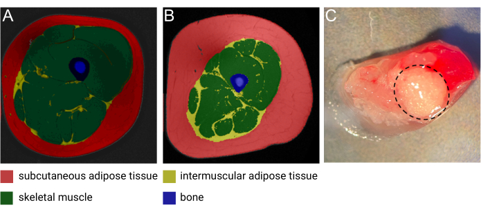
Figure 1: Images of IMAT. Representative magnetic resonance (MRI) image of IMAT from (A) a middle-aged lean female and (B) a middle-aged male with obesity. Red: subcutaneous adipose tissue, yellow: intermuscular adipose tissue, green: skeletal muscle, blue: bone. Image courtesy of Heather Cornnell, AdventHealth Translational Research Institute. (C) Fresh tissue sample with IMAT (encircled by dashed black line). Image courtesy of Meghan Hopf, AdventHealth Translational Research Institute and Bryan Bergman, University of Colorado. This figure has been modified with permission from Goodpaster et al.¹. Please click here to view a larger version of this figure.

A number of studies have been published from the livestock industry investigating the marbling of meat (IMAT in particular) in pigs, chickens, and cattle using single-cell (sc) and snRNA-seq¹⁰. These studies have identified several subpopulations of adipocytes and markers of potential progenitor cells of IMAT^11,12,13; however, whether these cellular compositions translate to human IMAT is unknown. To our knowledge, only one study has looked into the cellular heterogeneity of human muscle with fatty infiltration, obtained from male patients with hip osteoarthritis, using snRNA-seq¹⁴. The investigators reported a small adipocyte population and several fibro-adipogenic progenitor (FAP) subpopulations within the large population of myonuclei¹⁴. Our study is the first to develop a method to directly interrogate IMAT manually dissected from human muscle for cellular composition using snRNA-seq.

Importantly, protocols for snRNA-seq need to be customized for the specific tissue studied, as the amount of tissue available and the physical properties of the specific tissue will dictate the optimal processing steps. The tissue yield for IMAT is typically small, often not exceeding 50 mg, even when performing ultrasound-guided biopsies. Hence, proper processing of this scarce tissue is essential. We believe that this protocol will serve as a valuable resource for researchers studying human IMAT.

Protocol

The sample used for this protocol was part of the Study of Muscle, Mobility, and Aging (SOMMA)^15, which was approved by the Western IRB-Copernicus Group (WCG) Institutional Review Board and was carried out in accordance with the Declaration of Helsinki. Participants provided written informed consent for their participation in the study.

NOTE : This protocol is adapted from a previous protocol using 100 mg of human abdominal subcutaneous adipose tissue on a nanowell-based platform¹⁶. The current protocol is optimized for 50 mg of human IMAT and library preparation using a droplet-based platform. Further optimization of this protocol for nuclei isolations from non-human IMAT or other adipose depots may be required.

1. Preparation of buffers and reagents (Table 1 and Table 2)

NOTE: Prepare buffers fresh on the day of the experiment and do not re-use.

1. Pre-cool a centrifuge to 4 °C.
2. Prepare homogenization buffer and nuclei isolation medium.
   1. Obtain two buckets of ice and pre-cool 2 x 15 mL conical tubes.
   2. Mix all reagents for the homogenization buffer (HB) in a 15 mL conical tube in the order listed in Table 1. Keep on ice. Mix by vortexing.
   3. Mix all reagents for nuclei isolation medium (NIM) in a 15 mL conical tube in the ordered list in Table 2. Keep on ice. Mix by vortexing.
   4. Prepare 10% Triton-X by adding 100 µL of Triton X-100 to 900 µL of Nuclease-free water. Vortex to ensure proper mixing. Keep at room temperature (RT).

Reagent	Volume (μL)		Final concentration (mM)
	1x	2x
1 M MgCl2	10	20	5
1 M Tris Buffer, pH 8.0	20	40	10
2 M KCl	25	50	25
1.5 M Sucrose (-4oC)	334	668	250
1mM DTT	2	4	0.001 (~1 µM)
100x protease inhibitor	20	40	1x
Superasin 20 U/µL	40	80	0.4 U/µL
Nuclease-free water	1549	3098	-
Total Volume	2000	4000	-

Table 1: Homogenization buffer (HB). Keep on ice. Mix by vortexing.

Reagent	Volume (μL)		Final concentration (mM)
	1x	2x
EDTA	0.4	0.8	0.1
Ribolock RNAse inhibitor (40U/µL)	40	80	0.8 U/µL
1% BSA-PBS (-/-)	1959.6	3919.2	-
Total Volume	2000	4000	-

Table 2: Nuclei isolation medium (NIM). Keep on ice. Mix by vortexing.

2. Pulverization of frozen tissue ( Figure 2A)

1. Set up the workstation for homogenization.
   1. Fill up the cannister with liquid nitrogen (LN₂).
      CAUTION: when working with LN_2, always wear goggles and cryo gloves.
   2. Obtain 2x mortars, 1x pestle, 1x micro-scoop spatula, 1x glass dounce, and 1x stainless-steel pestle for the automatic douncer.
   3. Set up the automatic douncer.
   4. Fill a beaker with ice and pre-cool the glass dounce.
2. Fill the 2 mortars (containing the pestle and spatula) with LN₂ to cool down the instruments. Let the LN₂ evaporate and repeat.
3. While instruments are cooling, add 1 mL of HB to the glass dounce.
4. Fill both mortars with LN₂ one last time and pour the 50 mg IMAT sample into one of the mortars.
5. Pulverize the IMAT using the pestle by gently pressing it down on the piece of tissue to break it into small pieces. Make sure all pieces are pulverized.
6. The LN₂ will slowly evaporate while pulverizing the tissue. When tissue is properly pulverized, and there is still ¼ - ½ of a mortar of LN₂ left, tilt the mortar towards the lip of the mortar to collect the pulverized tissue by the lip. Let the LN₂ evaporate completely.
7. Immediately after the last LN₂ has evaporated, scoop the pulverized tissue into the glass dounce containing 1 mL of HB.

3. Homogenization of pulverized tissue

1. Homogenize the pulverized tissue using the automatic douncer. Bring the glass dounce up and down the stainless-steel pestle for 10 strokes in the forward direction, followed by 10 strokes in the reverse direction.
2. Ensure that the solution is cloudy after homogenization and contains no visible pieces of tissue. A light pink color is often expected due to contamination with muscle tissue.
3. Transfer the homogenate to a pre-cooled 1.7 mL low-bind tube on ice.
4. Use 400 µL of HB to rinse the dounce to make sure all the material is transferred and add it to the tube.
   NOTE: Two samples can be processed at a time. To do this, double the amount of HB and NIM. Pulverize and homogenize one tissue sample and immediately thereafter pulverize and homogenize the second tissue sample to be able to perform the isolation and clean-up steps in parallel.

4. Nuclei isolation and clean-up ( Figure 2B)

1. Add 14 µL of Triton-X (10%) to the homogenate for a 0.1% concentration.
2. Keep the tube on ice and in the dark for 10-15 min while vortexing every 3 min.
3. Pre-wet one 100 µm and one 40 µm cell strainer (per sample) with 100 µL of RT DPBS for each in a 50 mL conical tube.
4. Filter the homogenate through the 100 µm cell strainer.
5. Rinse the 1.7 mL tube with 400 µL of HB and filter through the 100 µm cell strainer.
6. Next, filter the solution through the 40 µm cell strainer.
7. Transfer an equal amount of solution into two pre-cooled 1.7 mL low-bind tubes corresponding to ~900 µL in each tube.
8. Centrifuge the tubes for 10 min at 2700 x g at 4 °C. There should be a small pellet visible after centrifugation.
9. Remove and discard the top lipid layer and the remaining supernatant, leaving ~50 µL solution from the first tube.
10. Repeat for the second tube.
11. Thoroughly resuspend the pellet in the first tube by gently pipetting up and down 20x and transfer to a new 1.7 mL low-bind tube. Avoid creating bubbles.
12. Repeat this procedure for the second tube and transfer the resuspended solution to the same tube.
13. Add 500 µL of NIM and mix with pipetting.
14. Centrifuge the tube with a balance at 1000 x g for 10 min at 4 °C.
15. Remove supernatant, leaving ~50 µL, and gently pipette up and down until the pellet is resuspended. Optionally, transfer the resuspended pellet to a new clean tube if some lipid leftover remains on the side of the tube.
16. Add 200 µL of NIM and mix by pipetting.

5. Nuclei staining and counting (Figure 2C and Figure 3)

NOTE : To facilitate the counting, set up a 'nuclei counting' protocol on an automated cell counter, as adjusting the bright field and DAPI channels can affect the count greatly. Adjust the channels so that only nuclei and not debris are captured. Make sure the bright field channel only marks 'objects' that also have a DAPI stain.

1. Add 1 drop of the live cell staining solution and leave it in the dark, on ice, for 15 min.
2. Filter the solution through a 30 µm cell strainer.
3. Mix the nuclei solution by pipetting and add 10 µL of the solution to a cell counting chamber slide.
4. Count nuclei using an automated cell counter.
   NOTE: The optimal concentration is 1000 nuclei/µL corresponding to 1.0 x 10⁶/mL.
   1. Ensure no clumps of nuclei are present, as this could clog the chip for generating single nuclei droplets (Figure 3).
   2. If the nuclei concentration is not high enough, spin down the solution at 1000 x g for 10 min at 4 °C to gain a pellet, remove the supernatant, and resuspend in a smaller volume.
   3. If the degree of debris in the solution is high, resuspend the nuclei solution in a larger volume of NIM (i.e., 1 mL) and filter through a 30 µm cell strainer again. Then spin down at 1000 x g for 10 min at 4 °C and resuspend in appropriate volume in relation to the concentration of nuclei.
5. After obtaining the nuclei concentration, proceed directly to the first step in the library preparation.

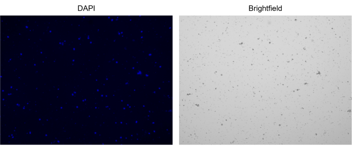
Figure 3: Staining of isolated nuclei. Image from cell counter of nuclei stained with NucBlue/DAPI (left image) and the corresponding bright field image (right image). The presence of minor amounts of debris is evident in the bright field image. The automated cell counter used here does not have an option to include scale bars. Please click here to view a larger version of this figure.

6. Library preparation and sequencing parameters

1. Refer to a thorough protocol for library preparation using the droplet-based single nuclei approach available on the provider's webpage¹⁷.
   1. Aim for a targeted nuclei recovery of 10,000. However, for samples with a high level of debris or fragile nuclei, a lower number of nuclei recovered would be anticipated.
   2. Store the samples at 4°C for up to 72 h after step 2.3. in the library preparation protocol to combine the processing of more samples in parallel. Do this by processing two samples until step 2.3 on two consecutive days, and on the third day, process the 4 samples together from step 3 and forward in the library preparation protocol.
2. Sequencing parameters: Sequence on a sequencing platform aiming for 50,000 paired-end reads per nuclei.
   ​NOTE: The data presented in this protocol was sequenced on the NovaSeq 6000 platform, aiming for 50,000 paired-end reads per nuclei.

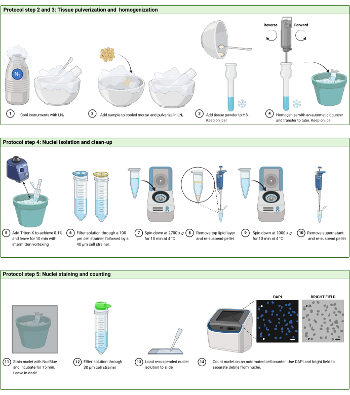
Figure 2: Protocol workflow. Schematic illustration of the workflow in (A) steps 2 and 3, (B) step 4, and (C) step 5 of the protocol. The figure was created with BioRender.com. Please click here to view a larger version of this figure.

7. Data processing and analysis

NOTE : In this protocol, some of the recommended software and R packages used to process the resulting sequencing data are briefly introduced, focusing on the steps after the initial pre-processing (Table 3). This study provides general quality control (QC) metrics and an example uniform manifold approximation and projection (UMAP) in Figure 4. However, an in-depth description of the bioinformatic analysis is out of the scope of this protocol. Therefore, readers can refer to the recent review on best practices for single-cell analysis by Heumos et al.¹⁸.

1. Pre-processing of sequencing data
   1. Map the single nuclei reads to the human reference genome GRCh38.
   2. Include intron reads in the count.
2. Perform QC and filtering of the data using the Seurat R package¹⁹.
   1. Compute a cell complexity score by dividing the log(10) number of genes detected by the log(10) number of reads detected.
   2. Plot out the most important QC metrics using a histogram or violin plot, including the number of genes detected per nuclei, mitochondrial read percentage, and cell complexity score.
   3. Filter out nuclei with less than 200 or more than 10,000 genes per nuclei, greater than 10% mitochondrial reads, and a complexity score below 0.8.
3. Normalize data and perform dimensionality reduction.
   1. Use the SCTransform function from Seurat to normalize the data using 2000 variable features.
   2. Cluster data using the following functions from the Seurat R package: RunPCA, FindNeighbors, FindClusters, and RunUMAP.
   3. Plot a UMAP to visualize the clustering of the data.
4. Filter out predicted doublets using the DoubletFinder R package²⁰ and re-cluster data.
5. Annotate clusters using known gene markers of the cell types expected to be present in the tissue (supervised approach) or based on the top 5 differentially expressed genes between the clusters (unsupervised approach).
6. Use decontX²¹ to determine the degree of ambient RNA contamination and to adjust the gene expression matrix for ambient RNA.
   1. Include the raw gene matrix as background.
7. Save the Seurat object for future exploration of the data.
   NOTE: The code for QC and clustering analysis is available in Supplementary File 1.

Software/R packages used in  data workflow	Alternative software/packages	Processing step
CellRanger	STARsolo, kallisto	Trimming, alignment, mapping
Seurat	SingleCellExperiment, Cellranger	QC, analysis and data exploration
DoubletFinder	scds, scdblFinder, Scrublet	Doublet detection
DecontX	SoupX, CellBender	Ambient RNA adjustment

Table 3: Software/tools for data workflow.

Results

This workflow was designed to guide the processing of frozen human IMAT samples to obtain gene expression profiles at single nuclei resolution, enabling cell type identification. Here, one representative IMAT sample from a participant in the SOMMA study is presented.

The first step of any analysis of snRNA-seq data is to evaluate the quality of the data to identify poor-quality nuclei, which should potentially be removed from the dataset. Importantly, the filtering steps and thresholds should ...

Discussion

There are several inherent challenges to working with IMAT. In addition to its limited accessibility, the yield of sample material is often very scarce, and "contamination" of skeletal muscle is almost impossible to avoid. To obtain the best quality sample, one should penetrate the muscle fascia when inserting the biopsy needle (to make sure not to collect subcutaneous adipose tissue) and remove as much muscle tissue as possible by dissecting the sample under a microscope immediately after collection, followed by...

Materials

List of materials used in this article

Name	Company	Catalog Number	Comments
0.2 µm corning syringe filters	Millipore Sigma	CLS431229
1.7 mL DNA LoBind tubes	Eppendorf	22431021	low-bind tubes
10% Tween 20	Bio-Rad	1662404
100x protease inhibitor	Thermo Fisher Scientific	78437
10X Magnetic Separator	10X Genomics	230003
10X Vortex Adapter	10X Genomics	330002
15 mL canonical tubes	Sarstedt	6,25,54,502
2100 Bioanalyzer	Agilent	G2939BA
50 mL conical tubes	Sarstedt	6,25,47,254
CellRanger	Genomics	N/A
Chromium iX accesory kit	10X Genomics	PN1000323
Chromium iX Controller	10X Genomics	PN1000326
Chromium Next GEM Chip G Single Cell Kit	10X Genomics	PN1000127
Chromium Next GEM Single Cell 3' Gel Bead Kit v3.1	10X Genomics	PN1000129
Chromium Next GEM Single Cell GEM Kit v3.1	10X Genomics	PN1000130
Countess 3 Automated Cell Counter	Thermo Fisher Scientific	AMQAX2000	Automated cell counter
Countess cell counting chamber slides	Thermo Fisher Scientific	C10228
DoubletFinder	R	N/A
DPBS (no calcium, no magnesium)	Thermo Fisher Scientific	14190144
DTT	Thermo Fisher Scientific	R0861
Dual Index Kit TT Set A, 96 rxns	10X Genomics	PN1000215
Dynabeads MyOne SILANE	10X Genomics	PN2000048
Falcon 100 µm Cell strainer	Corning Life Science	352360
Falcon 40 µm Cell strainer	Corning Life Science	352340
Glycerin (glycerol), 50% (v/v) Aqueous Solution	Ricca Chemical Company	3290-32
KCL	Thermo Fisher Scientific	AM9640G
Library Construction Kit v3.1	10X Genomics	PN1000196
MACS SmartStrainers (30µm)	Miltenyi Biotec	130-098-458
Mastercycler Nexus Gradient Thermal cycler	Eppendorf	6331000017
MgCl2	Ambion	AM9530G
Mortar and pestel	Health care logistics	14075
NucBlue Live Ready Probes Reagent	Thermo Fisher Scientific	R37605
Nuclease Free Water (not DEPC treated)	Thermo Fisher Scientific	AM9930
Probumin Bovine Serum Albumin Fatty Acid Free, Powder	Sigma-Aldrich	820024
Qiagen Buffer EB	Qiagen	19086
Ribolock RNAse inhibitor	Thermo Fisher Scientific	EO0382
Seurat	R	N/A
Sucrose	Sigma-Aldrich	S0389
SUPERasin 20 U/µL	Thermo Fisher Scientific	AM2695
ThermoMixer C	Eppendorf	5382000015
Tissue homogenizer	Glass-Col	099C K54
Tris buffer pH 8.0	Thermo Fisher Scientific	AM9855G
Triton X-100	Thermo Fisher Scientific	AC327372500
UltraPure 0.5M EDTA pH 8.0	Gibco	15575020

References

- Goodpaster, B. H., Bergman, B. C., Brennan, A. M., Sparks, L. M. Intermuscular adipose tissue in metabolic disease. Nat Rev Endocrinol. 19 (5), 285-298 (2023).
- Sparks, L. M., Goodpaster, B. H., Bergman, B. C. The metabolic significance of intermuscular adipose tissue: Is IMAT a friend or a foe to metabolic health. Diabetes. 70 (11), 2457-2467 (2021).
- Gallagher, D., et al. Adipose tissue in muscle: A novel depot similar in size to visceral adipose tissue. Am J Clin Nutr. 81 (4), 903-910 (2005).
- Manini, T. M., et al. Reduced physical activity increases intermuscular adipose tissue in healthy young adults. Am J Clin Nutr. 85 (2), 377-384 (2007).
- Addison, O., Marcus, R. L., LaStayo, P. C., Ryan, A. S. Intermuscular fat: A review of the consequences and causes. Int J Endocrinol. 2014, 309570(2014).
- Goodpaster, B. H., et al. Obesity, regional body fat distribution, and the metabolic syndrome in older men and women. Arch Intern Med. 165 (7), 777-783 (2005).
- Goodpaster, B. H., Thaete, F. L., Kelley, D. E. Thigh adipose tissue distribution is associated with insulin resistance in obesity and in type 2 diabetes mellitus. Am J Clin Nutr. 71 (4), 885-892 (2000).
- Goodpaster, B. H., et al. Association between regional adipose tissue distribution and both type 2 diabetes and impaired glucose tolerance in elderly men. Diabetes Care. 26 (2), 372-379 (2003).
- Sachs, S., et al. Intermuscular adipose tissue directly modulates skeletal muscle insulin sensitivity in humans. Am J Physiol Endocrinol Metab. 316 (5), E866-E879 (2019).
- Ford, H., Liu, Q., Fu, X., Strieder-Barboza, C. White adipose tissue heterogeneity in the single-cell era: From mice and humans to cattle. Biology (Basel). 12 (10), 1289(2023).
- Wang, L., et al. Single-nucleus and bulk RNA sequencing reveal cellular and transcriptional mechanisms underlying lipid dynamics in high marbled pork. NPJ Sci Food. 7 (1), 23(2023).
- Li, J., et al. Identification of diverse cell populations in skeletal muscles and biomarkers for intramuscular fat of chicken by single-cell RNA sequencing. BMC Genomics. 21 (1), 752(2020).
- Lyu, P., Qi, Y., Tu, Z. J., Jiang, H. Single-cell RNA sequencing reveals heterogeneity of cultured bovine satellite cells. Front Genet. 12, 742077(2021).
- Fitzgerald, G., et al. MME+ fibro-adipogenic progenitors are the dominant adipogenic population during fatty infiltration in human skeletal muscle. Commun Biol. 6 (1), 111(2023).
- Cummings, S. R., et al. The study of muscle, mobility and aging (SOMMA): A unique cohort study about the cellular biology of aging and age-related loss of mobility. J Gerontol A Biol Sci Med Sci. 78 (11), 2083-2093 (2023).
- Whytock, K. L., et al. Isolation of nuclei from frozen human subcutaneous adipose tissue for full-length single-nuclei transcriptional profiling. STAR Protoc. 4 (1), 102054(2023).
- 10x Genomics. Chromium Single Cell 3' Reagent Kits User Guide (v3.1 Chemistry Dual Index), Document Number CG000315 RevE. , Available from: https://cdn.10xgenomics.com/image/upload/v1668017706/support-documents/CG000315_ChromiumNextGEMSingleCell3-_GeneExpression_v3.1_DualIndex__RevE.pdf (2022).
- Heumos, L., et al. Best practices for single-cell analysis across modalities. Nat Rev Genet. 24 (1), 550-572 (2023).
- Hao, Y., et al. Dictionary learning for integrative, multimodal and scalable single-cell analysis. Nat Biotechnol. 42 (2), 293-304 (2023).
- McGinnis, C. S., Murrow, L. M., Gartner, Z. J. DoubletFinder: Doublet detection in single-cell RNA sequencing data using artificial nearest neighbors. Cell Syst. 8 (4), 329-337 (2019).
- Yang, S., et al. Decontamination of ambient RNA in single-cell RNA-seq with DecontX. Genome Biol. 21 (2), 57(2020).
- Common considerations for quality control filters for single cell RNA-seq data. 10X Genomics. , Available from: https://www.10xgenomics.com/analysis-guides/common-considerations-for-quality-control-filters-for-single-cell-rna-seq-data (2022).
- Luecken, M. D., Theis, F. J. Current best practices in single-cell RNA-seq analysis: a tutorial. Mol Syst Biol. 15 (6), e8746(2019).
- Emont, M. P., et al. A single-cell atlas of human and mouse white adipose tissue. Nature. 603 (7903), 926-933 (2022).
- Hildreth, A. D., et al. Single-cell sequencing of human white adipose tissue identifies new cell states in health and obesity. Nat Immunol. 22 (5), 639-653 (2021).
- Whytock, K. L., et al. Single cell full-length transcriptome of human subcutaneous adipose tissue reveals unique and heterogeneous cell populations. iScience. 25 (8), 104772(2022).
- Probst, V., et al. Benchmarking full-length transcript single cell mRNA sequencing protocols. BMC Genomics. 23 (1), 860(2022).
- CG000148 Rev A Technical Note - Resolving cell types as a function of read depth and cell number. Technical note. 10X Genomics. , Available from: https://assets.ctfassets.net/an68im79xiti/6gDArDPBTOg4IIkYEO2Sis/803be2286bb a5ca67f353e6baf68d276/CG000148_10x_Technical _Note_Resolving_Cell_Types_as_Function_of_ Read_Depth_Cell_Number_RevA.pdf (2018).
- Gupta, A., et al. Characterization of transcript enrichment and detection bias in single-nucleus RNA-seq for mapping of distinct human adipocyte lineages. Genome Res. 32 (2), 242-257 (2022).
- Bakken, T. E., et al. Single-nucleus and single-cell transcriptomes compared in matched cortical cell types. PLoS One. 13 (12), e0209648(2018).
- Wu, H., Kirita, Y., Donnelly, E. L., Humphreys, B. D. Advantages of single-nucleus over single-cell RNA sequencing of adult kidney: Rare cell types and novel cell states revealed in fibrosis. J Am Soc Nephrol. 30 (1), 23-32 (2019).
- Kim, N., Kang, H., Jo, A., Yoo, S. -A., Lee, H. -O. Perspectives on single-nucleus RNA sequencing in different cell types and tissues. J Pathol Transl Med. 57 (1), 52-59 (2023).
- Avila Cobos, F., Alquicira-Hernandez, J., Powell, J. E., Mestdagh, P., De Preter, K. Benchmarking of cell type deconvolution pipelines for transcriptomics data. Nat Commun. 11 (1), 5650(2020).
Access restricted. Please log in or start a trial to view this content.
Reprints and Permissions