Echocardiographic Assessment of Cardiac Anatomy and Function in Adult Rats

Summary

A non-invasive protocol for transthoracic echocardiography assessment of cardiac anatomy and function for adult rats is presented in the current study. The heart valves, all four cardiac chambers and the ascending aorta, aortic arch and descending aorta are studied in detail.

Abstract

The use of experimental animal models has become crucial in cardiovascular science. Most studies using rodent models are focused on two-dimensional imaging to study the cardiac anatomy of the left ventricle and M-mode echo to assess its dimensions. However, this could limit a comprehensive study. Herein, we describe a protocol that allows an assessment of the heart chamber size, left ventricular function (systolic and diastolic) and valvular function. A conventional medical ultrasound machine was used in this protocol and different echo views were obtained through left parasternal, apical and suprasternal windows. In the left parasternal window, the long and short axis were acquired to analyze left chamber dimensions, right ventricle and pulmonary artery dimensions, and mitral, pulmonary and aortic valve function. The apical window allows the measurement of heart chamber dimensions and evaluation of systolic and diastolic parameters. It also allows Doppler assessment with detection and quantification of heart valve disturbances (regurgitation or stenosis). Different segments and walls of the left ventricle are visualized throughout all views. Finally, the ascending aorta, aortic arch, and descending aorta can be imaged through the suprasternal window. A combination of ultrasound imaging, Doppler flow and tissue Doppler assessment have been obtained to study cardiac morphology and function. This represents an important contribution to improve the assessment of cardiac function in adult rats with impact for research using these animal models.

Introduction

Cardiovascular disease is the leading cause of death in Europe, responsible for over 4 million yearly deaths, despite advances in therapy, diagnosis, and monitoring that have improved patient outcomes in recent years. A rapid technological evolution has contributed to progress in cardiovascular patient care. Within these diagnostic tools, particular attention has been paid to biomedical imaging, which allows an anatomic and functional evaluation in a non-invasive way^1,2,3. Similarly, medicine benefits from the results of biomedical research. Experimental animal models are very useful for testing hypotheses derived from the clinical setting and to develop innovative therapies^4,5.

There is increasing interest in the use of echocardiography as a research tool in experimental animal models, allowing the acquisition of multiple measurements from a single animal in longitudinal studies. It is important to note that there are some advantages in using murine or rodent models. The short gestation period, low cost of breeding and housing, the knowledge of their genome and possibility to develop transgenic animals are the main advantages of these species, making them attractive to study the mechanisms involved in cardiovascular disease^4,5,6,7,8,9. Although rat and mouse models show similar advantages, rats are the classical choice in cardiovascular studies due to their larger physical dimension and lower heart rate that provides better images in echocardiography studies^{4,5,6,7,8,9,10}.

We describe an echocardiography protocol using conventional medical ultrasound equipment to evaluate cardiac chambers and heart valves (anatomy and function) using Wistar rats. This is a concise and complete protocol for short time acquisition images and loops that allow offline measurements, which can be later revised to integrate new variables or measurements over time.

Protocol

All animal procedures were performed according to Directive 2010/63/EU. The procedures were approved by the institutional Animal Welfare Body, licensed by DGAV, the Portuguese competent authority for animal protection (license number 0421/000/000/2018).
NOTE: Female Wistar Han IGS (Crl:WI(Han) from Charles River Laboratories (12-16 weeks-old) were used. This protocol is specific for rats independently of their strain, age or gender.

1. Preparing Rats for Echocardiography: Anesthesia and Reversion Protocol

1. Weigh rats.
2. Prepare a three-component anesthetic composed by midazolam (4.76 mg/kg), medetomidine (0.356 mg/kg) and fentanyl (0.012 mg/kg), according to rat weight.
3. Inject anesthesia intraperitoneally. Check for the absence of pedal withdrawal reflexes to evaluate the depth of anesthesia.
4. Shave the hair from the torso area.
5. Apply durable gel to both eyes to prevent drying of the sclera.
6. Place the anesthetized rat in a supine position atop a heating pad in order to maintain body temperature (37.0 °C ± 0.5 °C).
7. Apply a layer of preheated (close to body temperature) ultrasound gel to the chest, mainly in the area overlying the heart. Avoid air bubbles in the gel that can interfere with ultrasonic imaging.
8. Reverse anesthesia through subcutaneous injection using atipamezole (0.94 mg/kg) and flumazenil (0.2532 mg/kg), immediately after the end of the echocardiography.
   NOTE: This anesthetic combination provides up to 45 min for echocardiography imaging. The echocardiographic protocol described below is compatible with any other anesthesia protocol.

2. Echocardiography

NOTE: The echocardiograms are performed with a conventional clinical echocardiographic equipment, with a 12 MHz cardiac probe, and include acquired still images and loops in parasternal (long axis and short axis views), apical (4, 5, 2 and 3 chambers) and suprasternal views. An electrocardiogram is recorded to identify end-systole and end-diastole, for measurement procedures and loop acquisition (ECG triggered)^11,12. A preset is used to keep image definition stable between rats: frequency 5-10 MHz, depth 2.5 cm, frame rate 125 fps, Doppler sample 1.0 mm and color Doppler aliasing velocity 40 cm/s. Loops were recorded with at least 3 heart beats.

1. Left parasternal long axis view
   NOTE: Position the probe on the left side of the sternum and the index mark turned to the right shoulder.
   1. Record M-mode images at the aortic valve, mitral valve leaflets and left ventricular mid-cavity (cursor at mitral valve tips or cordal level)^1,2,3,4. The M-Mode cursor should be perpendicular to the structure of interest^1,3,10.
   2. Record a 2D loop of all views.
   3. Record a 2D loop with zoom at the left ventricular outflow tract.
   4. Record a 2D loop with color Doppler imaging simultaneously at the aortic and mitral valves.
2. Left parasternal short-axis view
   NOTE: Place the probe on the left side of the sternum with the index mark rotated to the left shoulder.
   1. Obtain an image at the aortic valve level by tilting the probe slightly cranially.
   2. Record a 2D loop of all views.
   3. Record a 2D loop with color Doppler imaging simultaneously at the aortic and pulmonary valves.
   4. Acquire a spectral pulsed Doppler image at the pulmonary artery. The cursor should be parallel to flow^1,3.
   5. Obtain an image of the left ventricle at the papillary muscle level by tilting the probe slightly downward.
   6. Record a 2D loop of all views.
3. Apical 4-chamber view
   NOTE: Position the probe at the apical area in the anterior axillary line and with the index mark turned to left shoulder.
   1. Record a 2D loop of all views.
   2. Record a loop of 2D and tissue Doppler imaging including all 4 chambers.
   3. Focus on the left cardiac chambers.
      1. Record a 2D loop with zoom at the left atrium.
      2. Record a 2D loop with color Doppler imaging at the mitral valve and left atrium.
      3. Record simultaneous M-mode and color Doppler images for left ventricular propagation flow.
      4. Get a spectral pulsed wave (PW) Doppler at the mitral valve for left ventricular inflow. Place the sample at the mitral leaflet tips, in their fully open diastolic position^1,2,3,11,12.
      5. Add a continuous wave (CW) Doppler image at the mitral valve, if there is mitral valve regurgitation.
      6. Obtain a spectral pulsed tissue Doppler image at the mitral annulus (left ventricular lateral and septal walls). Align the PW Doppler cursor with the long axis of the heart in order to produce the maximum Doppler signal^1,2,3,13.
      7. Record M-mode of mitral annulus for mitral annular plane systolic excursion measurement (cursor at lateral left ventricle wall).
   4. Focus on right cardiac chambers.
      1. Record a 2D loop with zoom at the right atrium.
      2. Record a 2D loop with color Doppler imaging at the tricuspid valve and the right atrium.
      3. Obtain a spectral pulsed tissue Doppler image at the tricuspid annulus (right ventricular wall).
      4. Record M-mode for tricuspid annular plane systolic excursion (TAPSE) by placing the 2D cursor at the tricuspid lateral annulus.
4. Apical 5-chamber view
   NOTE: From the 4-chamber view, tilt the probe slightly anterior to the chest.
   1. Record a 2D loop of all views.
   2. Record a 2D loop with color Doppler imaging at the aortic valve and left ventricular outflow tract.
   3. Get a spectral pulsed wave Doppler image at the left ventricular outflow tract. Place the cursor parallel to the flow and place the sample at the left ventricular outflow tract^4,14.
   4. Get a spectral pulsed wave Doppler image at the left ventricle mid-cavity for simultaneous left ventricular inflow and outflow waves.
   5. Obtain a spectral continuous wave Doppler image at aortic valve. Transvalvular flow is recorded below baseline and regurgitation, if present, above baseline.
5. Apical 2-chamber view
   NOTE: Return to a 4-chamber view and rotate the probe 90° counterclockwise.
   1. Record a 2D loop of all views.
   2. Record a 2D loop with color Doppler imaging at the mitral valve.
6. Apical 3-chamber view
   NOTE: Tilt the probe slightly cranially.
   1. Record a 2D loop of all views.
   2. Record a 2D loop with color Doppler simultaneously at the aortic and mitral valves.
7. Suprasternal window
   NOTE On the left side of supraclavicular space with probe directed downward
   1. Record a 2D loop of the aortic arch.
   2. Get spectral pulsed wave Doppler image at the ascending aorta.
   3. Get spectral pulsed wave Doppler image at the descending aorta.

3. Measurements

1. Proceed to measurements, including global longitudinal strain. Perform these measurements offline in order to reduce the anesthesia time.

Results

Figure 1 shows the probe position on the chest to display the parasternal window long axis view (Figure 2). This view allows accurate measurements of left ventricle cavity and wall thickness, systolic function (Figure 3), left ventricle outflow diameter (to apply in other formulas such as in cardiac output), ascending aorta diameter and left atrium diameter. All chamber dimensions were indexed to body weight. The parasternal long axis view allows anatomical (with 2D-Echo) and functional (with color Doppler imaging) evaluation of the aortic and mitral valves. This view also allows the identification and measurement of the pericardial effusion, if present. M-Mode can be used for left ventricle measurements (Figure 3): septum and posterior walls dimensions, left ventricle dimensions, left ventricle systolic function and left ventricle mass^1,3,4,10,14.

Left ventricle systolic function is evaluated by fractional shortening and also by visualizing the excursion and thickening of walls during cardiac cycle (assessed by the ECG). Left ventricle mass is obtained by the formula:
LV mass = 0.8 x 1.04 x [(IVS + LVID + PWT)³ - LVID³]
(IVS: interventricular septum thickness; LVID: left ventricle internal diameter; PWT: posterior wall thickness, with measurements made at end-diastole)^1,3,4,10,14.

Figure 4 shows the probe position on the chest to display the parasternal window short axis view. This view allows the visualization of the right ventricular outflow, the aortic valve, the pulmonary valve, the pulmonary artery (Figure 5), and the left ventricular mid-cavity size (Figure 6) and function (with 2D visualization of segmental contractility)^1,3,4,10,11.

Figure 7 shows the probe position on the chest to display the apical views. In the apical 4-chamber view (Figure 8), all 4-chamber dimensions (areas of all 4-chambers and volume of left ventricle) and function can be assessed. The anatomic and functional characterization of mitral and tricuspid valves can be also evaluated. The left ventricular outflow, aortic valve flow and ascending aorta were obtained with the apical 5-chamber view. The apical 2-chamber view (Figure 9) focuses on the left atrium and ventricular size and function. Apical 3-chamber and 5-chamber views allow aortic valve and left ventricular outflow evaluation. All views combined to allow the assessment of the different left ventricular walls and segments and the study of different systolic and diastolic function parameters^1,3,4,10,11.

Left ventricular diastolic function can be assessed by pulsed Doppler imaging at the mitral valve (Figure 10), isovolumetric relaxation time of the left ventricle, and tissue Doppler imaging at the mitral annulus^1,3,12. Normal mitral inflow consists of biphasic flow from the left atrium to the left ventricle. In normal conditions, the early flow coincident with E-wave is higher than the later flow that occurs with atrial contraction (A-wave).

Left ventricular diastolic function can also be studied with tissue Doppler imaging, which analyzes myocardial velocities (Figure 11). Spectral tissue Doppler imaging studies systolic and diastolic function over a cardiac cycle and has 3 peaks: one positive systolic peak (s'-wave) representing myocardial contraction and two negative diastolic peaks (e'-wave of early diastolic myocardial relaxation and a'-wave of active atrial contraction in late diastole) assessed at the mitral annular level, from septal or lateral annulus^1,3,4,10,14.

Characterization of left ventricular diastolic function by pulsed Doppler imaging at the mitral valve and tissue Doppler imaging at the mitral annulus should include the following parameters: E-wave velocity, A-wave velocity, E/A ratio, e' velocity, a' velocity, E/e' ratio and deceleration time of E-wave^1,3,4,10,14.

Left ventricular systolic function can be studied by mitral annular plane systolic excursion measurement, fractional shortening (Figure 3), ejection fraction, stroke volume, cardiac output, systolic tissue s'-wave velocity (Figure 11) and global longitudinal strain by myocardial deformation with strain and strain rate analysis (Figure 12)^1,3,4,10.

Ejection fraction is calculated with volumes by a modified Simpson method based on visual tracings of the blood and tissue interface using the apical 4 and 2-chamber views. At the basal or mitral valve level, the contour is closed by connecting the two opposite sections of the mitral ring with a straight line^1,3,4,10. The volume of blood that forms the ejection fraction represents the stroke volume. If the mitral valve is competent, then this can be multiplied by heart rate to calculate the cardiac output^1,3,4. Stroke volume is based on the measurements of blood flow through the left ventricle outlet tract during cardiac cycle, using this formula:
SV = π x (LVOT diameter /2)² x VTI _(LVOT)
(LVOT: left ventricle outflow tract; LVOT diameter is measured in the parasternal long axis view. VTI_(LVOT): velocity time integral traced from pulsed wave Doppler at LVOT in apical 5-chamber view)^1,3.

The most commonly used strain-based measure of LV global systolic function is global longitudinal strain obtained by myocardial deformation with strain and strain rate analysis^1,3,4,10. It is usually assessed by speckle-tracking echocardiography, where the peak of global longitudinal strain describes the relative length change of the LV myocardium between end-diastole and end-systole:
GLS(%) = (MLs − MLd)/MLd
(MLs: myocardial length at end-systole; MLd: myocardial length at end-diastole).

Measurements should begin with the apical 3-chamber view to visualize aortic valve closure, using opening and closing clicks of the aortic valve in spectral Doppler imaging or aortic valve opening and closing on M-mode imaging^1,3,4,10. Apical 4 and 2-chamber views are also evaluated, and all three views' measurements are averaged. Right ventricular systolic function is evaluated by tricuspid annular plane systolic excursion (TAPSE) and tissue Doppler imaging at tricuspid annulus. All valves are studied by color Doppler imaging, allowing direct visualization of stenosis or regurgitation (Figure 13). If aortic valve regurgitation is present, it can be studied and quantified by vena contracta and half-pressure time with continuous Doppler imaging (Figure 14)¹⁵. Figure 15 shows the ascending aorta, the aortic arch and the proximal descending aorta visualized in suprasternal window.

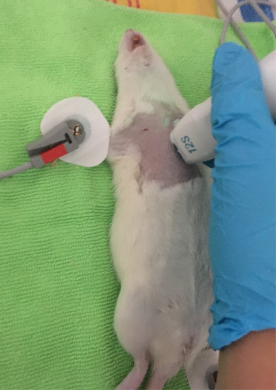
Figure 1: Probe positioning for parasternal long-axis view. Please click here to view a larger version of this figure.

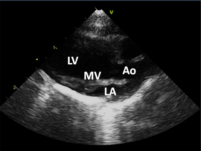
Figure 2: 2D parasternal long-axis view of left atrium (LA), left ventricle (LV), aortic valve, ascending aorta (Ao) and mitral valve (MV). Please click here to view a larger version of this figure.

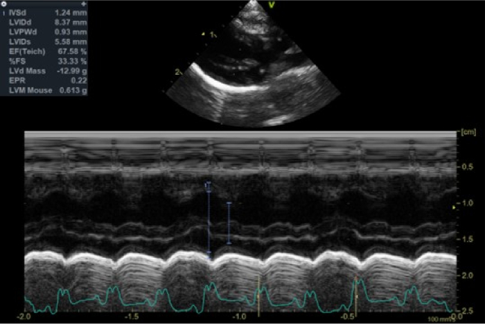
Figure 3: M-Mode of left ventricle with measurements, including interventricular septum thickness in diastole (IVSd), left ventricle internal diameter in diastole (LVIDd) and systole (LVIDs), posterior wall thickness (LVIPWd), fractional shortening (%FS), ejection fraction calculated with Teichholz method [EF(Teich)], left ventricle mass (LVdMass), parietal thickness (EPR) and left ventricle mass with calculation adapted to rodent (LVM Mouse). Please click here to view a larger version of this figure.

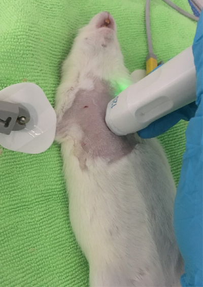
Figure 4: Probe positioning for parasternal short-axis view. Please click here to view a larger version of this figure.

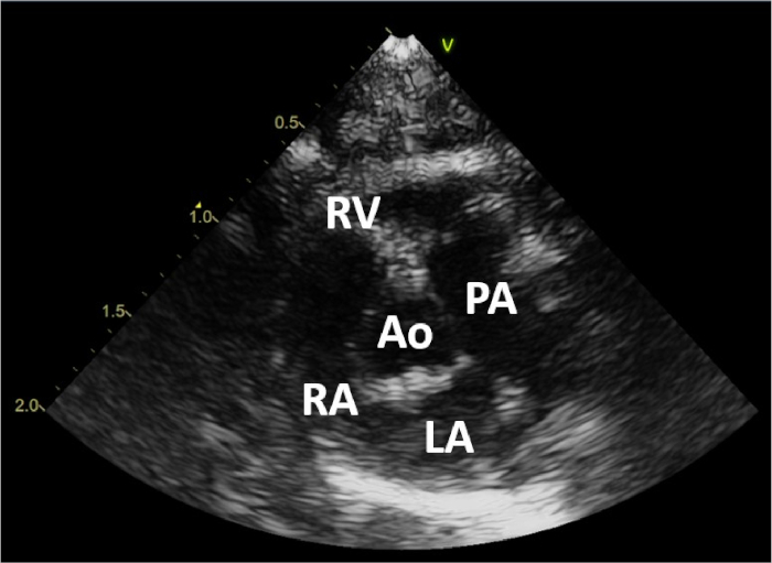
Figure 5: 2D parasternal short-axis view at aortic valve (Ao), left atrium (LA), right atrium (RA), right ventricle (RV) and pulmonary artery (PA). Please click here to view a larger version of this figure.

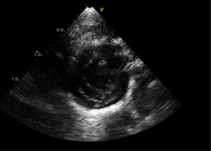
Figure 6: Parasternal short-axis view at left ventricle papillary muscles level. Please click here to view a larger version of this figure.

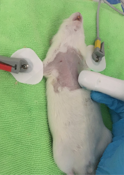
Figure 7: Probe positioning for apical 4-chamber view. Please click here to view a larger version of this figure.

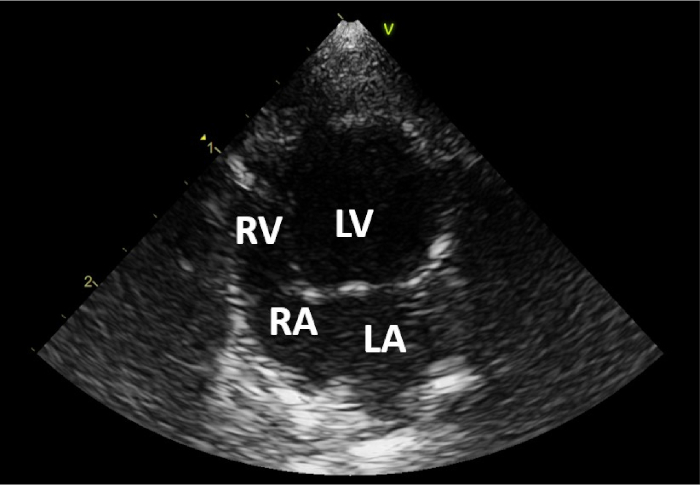
Figure 8: 2D of 4-chamber view including left atrium (LA), left ventricle (LV), right atrium (RA) and right ventricle (RV). Please click here to view a larger version of this figure.

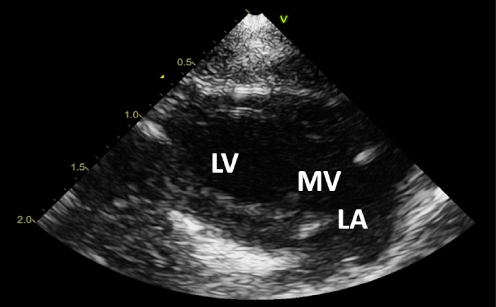
Figure 9: 2D Echo of apical 2-chamber view including left atrium (LA), ventricle (LV) and mitral valve (MV). Please click here to view a larger version of this figure.

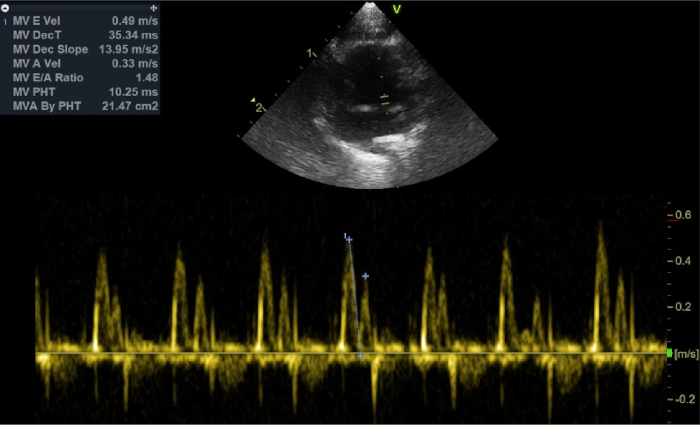
Figure 10: Pulsed wave Doppler at mitral valve, showing E-wave velocity = 0.49 m/s, A-wave velocity = 0.33 m/s, E-wave deceleration time = 35 ms and E/A ratio = 1.48. Please click here to view a larger version of this figure.

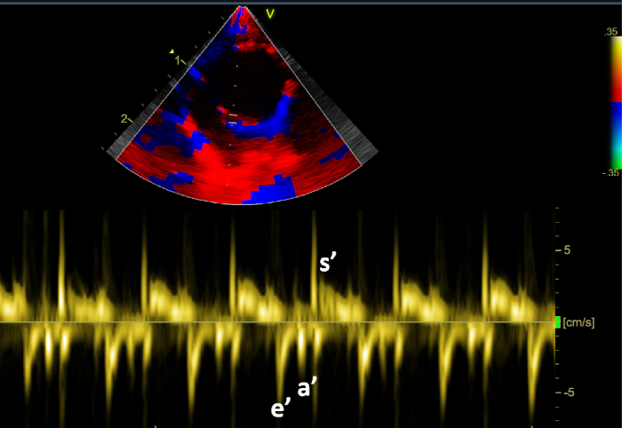
Figure 11: Spectral Doppler tissue at septal mitral annulus, showing myocardial tissue waves of diastole (e' and a') and of systole (s'). Please click here to view a larger version of this figure.

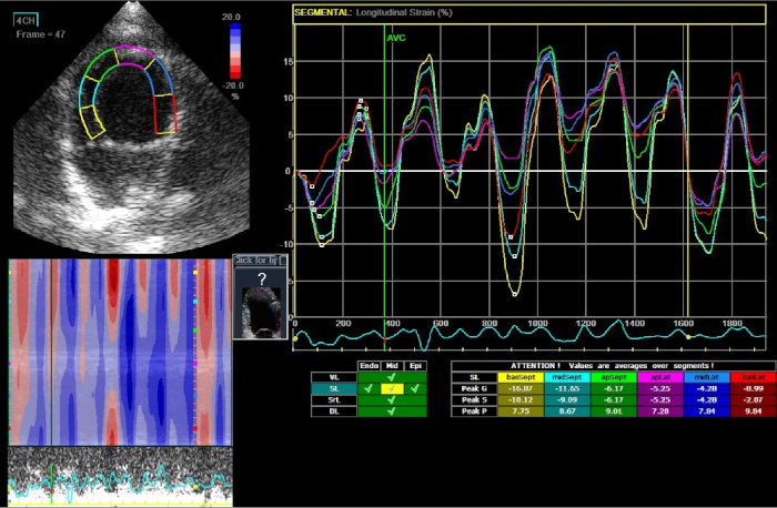
Figure 12: Myocardial deformation analysis with longitudinal strain evaluated at 4-chamber view. Please click here to view a larger version of this figure.

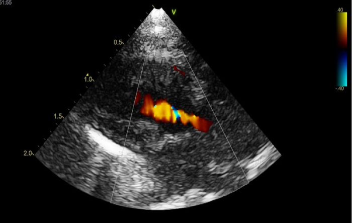
Figure 13: Visualization of aortic regurgitation with Color Doppler. Please click here to view a larger version of this figure.

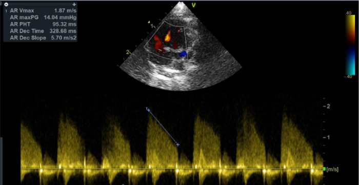
Figure 14: Continuous Doppler of aortic valve at apical 5-chamber view, showing regurgitation above baseline with half-pressure time measured of 95 ms. Please click here to view a larger version of this figure.

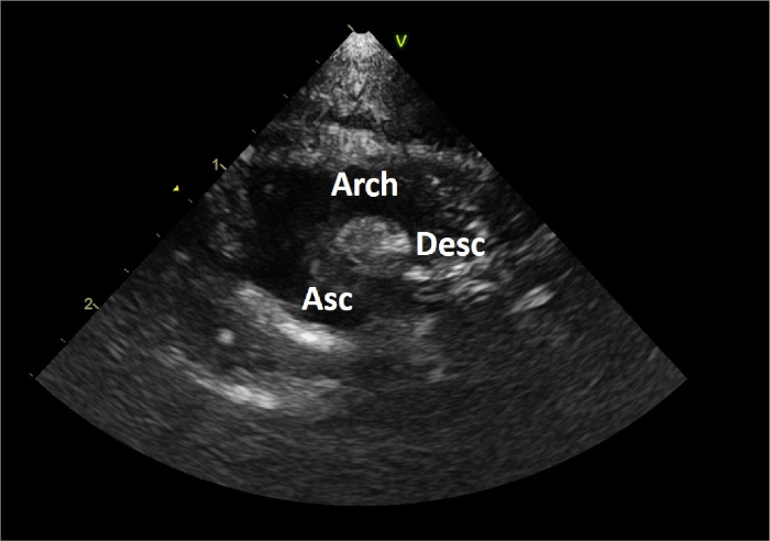
Figure 15: Suprasternal view of ascending aorta (Asc), aortic arch (Arch) and descending aorta (Desc). Please click here to view a larger version of this figure.

Discussion

This protocol allows a complete echocardiographic study using conventional medical ultrasound equipment and a high-frequency probe in adult rats. This is an important aspect of the protocol, since ultrasound equipment dedicated for small animals is expensive and the investment is not always justifiable.

As longitudinal imaging studies require repeated anesthesia, a combination of medetomidine-midazolam-fentanyl was proposed in this protocol since it is more suitable for serial use when compared to isoflurane or a mixture of ketamine-xylazine, in Wistar rats. However, the proposed echocardiographic protocol is compatible with any other anesthesia protocol¹⁶. As described, our echocardiography protocol includes the evaluation of several parameters that enables the identification of anatomic and functional cardiac changes.

Focusing on the anatomical characterization, it is possible to evaluate the dimensions of all heart chambers and their dilatations, left ventricle hypertrophy, valvular fibrosis or calcifications. Concerning the cardiac function, the left ventricular systolic and diastolic function and right ventricular systolic function can be analyzed^1,3,4. Also, the cardiac valve's anatomy and function are studied, using 2D-echo for anatomic characterization (identifying fibrosis, calcification or abnormal opening) and using Doppler imaging for functional characterization and detection of stenosis or regurgitations. Color Doppler imaging enables detection of flow direction and turbulences and spectral Doppler waves allow measurements of velocities and gradients^1,3.

Adequate image quality was obtained in almost all rats (smallest weight of 200 g), although due to inter-individual differences in anatomy, echocardiographic views may not be obtained with the exact same definition between rats, which may have an impact in cavity dimension measurements. There is 5% intra-observer reported variability on left ventricle M-mode measurements¹⁷. Particularly, when using M-Mode for left ventricular measurements, the following limitations may exist: difficulties in getting a perpendicular angle; including only basal segments (resulting in inaccurate measurements in the presence of asymmetric hypertrophy or regional systolic dysfunction); and geometric assumptions (considering that the left ventricle is a prolate ellipsoid with a 2:1 long/short axis ratio and symmetric distribution of hypertrophy). Also, inclusion of cubed measurements may impact accuracy, since even a small error in dimensions may lead to overestimated mass^1,3,10. Even when using volumes and the ejection fraction calculated by the Simpson's method, there are disadvantages: the apex is frequently foreshortened; the endocardial dropout can bias the measurement and is blind to shape distortions not visualized in the apical 4 and 2-chamber views^1,3,10.

Importantly, this protocol highlights the use of advanced measurements and evaluations, such as the left ventricle strain and the strain rate, assessed by speckle tracking, to achieve more complete information about myocardial fibers behavior^1,3. For a more accurate strain and strain rate evaluation, the optimization of image quality, maximizations of frame rate, and minimization of apex foreshortening are required. Midwall global longitudinal strain is used as it agrees with more published available data and has been shown in several clinical studies to be robust and reproducible¹⁰. The electrocardiographic monitorization integrated in the equipment is very prone to artifacts, which is a constraint. Also, it is very important to state that the functional or hemodynamic cardiac status of the rat can depend on variables such as temperature, blood pressure and heart rate^{4,5,6,7,8,9,13,14,17}.

Since resolution is related to the probe-frequency, future developments are expected to develop higher frequency probes and consequently higher resolution and image definition in non-invasive cardiovascular imaging in small animals, with this type of equipment. Standardization of methods and measurements is considered critical in this field of research, reaching more precise echocardiographic diagnosis of experimental rat models and resulting in a better understanding of molecular biology of human cardiovascular diseases.

Materials

List of materials used in this article

Name	Company	Catalog Number	Comments
12S-RS Probe	GE Medical Systems	H44901AB
Antisedan (5 mg/mL)	Esteve	P01B9003
EKG monitoring unit	GE Medical Systems	N/A
Electrodes	FIAB	F9089/100
Fentanilo (0.05 mg/mL)	B.Braun	BB3644960
Flumazenilo (0.1 mg/mL)	Generis	MUEH5933080
Insuline Syringe 1 mL	SOL M	1612912
Lubrithal gel (10 mg)	Dechra	NC519
Medetor (1 mg/mL)	Vibarc	P01B0308
Midazolan (5 mg/mL)	Labesfal	MUEH5506191
Shaver Razor AESCULAP Isis GT608	Braun	90200714
Small Animal Heated Pad 120 V	K&H Manufacturing inc.	655199010608
Ultrasound Gel	Parker Laboratories	REF 01-08
Ultrasound machine	GE Medical Systems	VIVID T8
Underpads	Henry Schein	900-8132

References

- Armstrong, W. F., Ryan, T. Feigenbaum's Echocardiography. , 7th Edition, Lippincott Williams & Wilkins. (2010).
- Douglas, P. S., et al. ACCF/ASE/ACEP/ASNC/SCAI/SCCT/SCMR 2007 appropriateness criteria for transthoracic and transesophageal echocardiography: a report of the American College of Cardiology Foundation Quality Strategic Directions Committee Appropriateness Criteria Working Group, American Society of Echocardiography, American College of Emergency Physicians, American Society of Nuclear Cardiology, Society for Cardiovascular Angiography and Interventions, Society of Cardiovascular Computed Tomography, and the Society for Cardiovascular Magnetic Resonance endorsed by the American College of Chest Physicians and the Society of Critical Care Medicine. Journal of the American College of Cardiology. 50 (2), 187-204 (2007).
- Otto, M. C. Textbook of Clinical Echocardiography. , 6th Revised Edition, Elsevier - Health Sciences Division. (2018).
- Liu, J., Rigel, D. F. Echocardiographic examination in rats and mice. Cardiovascular Genomics. Methods in Molecular Biology (Methods and Protocols). 573, 139-155 (2009).
- Ram, R., Mickelsen, D. M., Theodoropoulos, C., Blaxall, B. C. New approaches in small animal echocardiography: imaging the sounds of silence. American Jounal of Physiology- Heart and Circulatory Physiology. 301 (5), H1765-H1780 (2011).
- Aronsen, J. M., et al. Noninvasive stratification of postinfarction rats based on the degree of cardiac dysfunction using magnetic resonance imaging and echocardiography. American Jounal of Physiology - Heart and Circulatory Physiology. 312 (5), H932-H942 (2017).
- Forman, D. E., Cittadini, A., Azhar, G., Douglas, P. S., Wei, J. Y. Cardiac morphology and function in senescent rats: gender-related differences. Journal of the American College of Cardiology. 30 (7), 1872-1877 (1997).
- Walker, E. M. Jr, et al. Age-associated changes in hearts of male Fischer 344/Brown Norway F1 rats. Annals Of Clinical And Laboratory Science. 36 (4), 427-438 (2006).
- Watson, L. E., Sheth, M., Denyer, R. F., Dostal, D. E. Baseline echocardiographic values for adult male rats. Journal of the American Society of Echocardiography. 17 (2), 161-167 (2004).
- Lang, R. M., et al. Recommendations for cardiac chamber quantification by echocardiography in adults: an update from the American Society of Echocardiography and the European Association of Cardiovascular Imaging. Journal of the American Society of Echocardiography. 28 (1), 1-39 (2015).
- Galderisi, M., et al. Standardization of adult transthoracic echocardiography reporting in agreement with recent chamber quantification, diastolic function, and heart valve disease recommendations: an expert consensus document of the European Association of Cardiovascular Imaging. European Heart Journal - Cardiovascular Imaging. 18 (12), 1301-1310 (2017).
- Nagueh, S. F., et al. Recommendations for the Evaluation of Left Ventricular Diastolic Function by Echocardiography: An Update from the American Society of Echocardiography and the European Association of Cardiovascular Imaging. European Heart Journal - Cardiovascular Imaging. 29 (4), 277-314 (2016).
- Weytjens, C., et al. Doppler myocardial imaging in adult male rats: reference values and reproducibility of velocity and deformation parameters. European Journal of Echocardiography. 7 (6), 411-417 (2006).
- Scheer, P., et al. Basic values of M-mode echocardiographic parameters of the left ventricle in outbreed Wistar rats. Veterinarni Medicina. 57 (1), 42-52 (2012).
- Lancellotti, P., et al. Recommendations for the echocardiographic assessment of native valvular regurgitation: an executive summary from the European Association of Cardiovascular Imaging. European Heart Journal - Cardiovascular Imaging. 14 (7), 611-644 (2013).
- Albrecht, M., Henke, J., Tacke, S., Markert, M., Guth, B. Influence of repeated anaesthesia on physiological parameters in male Wistar rats: a telemetric study about isoflurane, ketamine-xylazine and a combination of medetomidine, midazolam and fentanyl. BMC Veterinary Research. 10, 310(2014).
- Dragoi Galrinho, R., et al. New Echocardiographic Protocol for the Assessment of Experimental Myocardial Infarction in Rats. Maedica (Bucharest). 10 (2), 85-90 (2015).
Reprints and Permissions