Metabolic Profiling to Determine Bactericidal or Bacteriostatic Effects of New Natural Products using Isothermal Microcalorimetry

Summary

The elucidation of the mode-of-action of a novel antibiotic is a challenging task in the drug discovery process. The goal of the method described here is the application of isothermal microcalorimetry using calScreener in antibacterial profiling to provide additional insight into drug-microbe interactions.

Abstract

Due to the global threat of rising antimicrobial resistance, novel antibiotics are urgently needed. We investigate natural products from Myxobacteria as an innovative source of such new compounds. One bottleneck in the process is typically the elucidation of their mode-of-action. We recently established isothermal microcalorimetry as part of a routine profiling pipeline. This technology allows for investigating the effect of antibiotic exposure on the total bacterial metabolic response, including processes that are decoupled from biomass formation. Importantly, bacteriostatic and bactericidal effects are easily distinguishable without any user intervention during the measurements. However, isothermal microcalorimetry is a rather new approach and applying this method to different bacterial species usually requires pre-evaluation of suitable measurement conditions. There are some reference thermograms available of certain bacteria, greatly facilitating interpretation of results. As the pool of reference data is steadily growing, we expect the methodology to have increasing impact in the future and expect it to allow for in-depth fingerprint analyses enabling the differentiation of antibiotic classes.

Introduction

The aim of this method is to apply isothermal microcalorimetry (IMC) as a medium throughput assay in mode-of-action (MoA) profiling of new antibacterial compounds. This method reveals data regarding the activity of compounds on bacterial species and provides information on the bactericidal or bacteriostatic nature of the compound itself.

The rise of emerging antimicrobial resistance (AMR) is a global problem and it leads to less effective treatments of common infections with known antibiotics¹. However, the search for new compounds and drugs that can replace or work in combination with known antibiotics are ongoing and this is built on diverse approaches. Natural products are a key player in current drug discovery campaigns and particularly in anti-infective drug discovery². However, identifying new lead structures for antibiotic development is a lengthy and financially demanding process³. Thus, the early steps of discovery are extremely important in order to filter on most promising scaffolds already at an early stage. Initial steps in natural product drug discovery include obtaining a compound’s structure, determining the activity in vitro along with MoA and target identification. Most successful compounds being eligible for further development should display a favorable spectrum of activity (i.e., broad-spectrum activity in the case of antibacterials) and a novel MoA by which pre-existing AMR can be overcome. Promising scaffolds are then typically screened in secondary assays, which include in vivo bioavailability, toxicity, and metabolism⁴. Besides the financial concerns, natural product drug discovery faces further challenges concerning the costs and technical difficulties related to compound isolation and purification, which, in turn, can make it difficult to obtain multi-milligram or even gram amounts in the early stages of the discovery process^5,6. Therefore, it is of utmost importance in natural product research to be able to perform state-of-the-art primary screening with minimal compound amounts in order to take a well-informed decision about further investments to make a novel natural product accessible for pre-clinical development. With the use of IMC for antibacterial profiling, the amount of compound needed is significantly reduced in comparison to standard methods. The technique also provides more in-depth information regarding the interaction of new drugs with the microbial community⁷.

IMC is a well-established method for measuring total energy as a result of all biological, physical and biochemical processes and reactions in a biological system. Bacterial energy release is proportional to the total metabolic reactions⁸. Within a closed system, such as the used microcalorimeter, the heat levels can be measured in the microwatt range to study the metabolic kinetics of bacteria^9,10,11,12. The heat (energy) that is released by bacteria is linked to cellular functions that underlie their metabolism and that are not necessarily proportional to the cellular biomass.

Initially, the applicability of isothermal calorimetry for microbiological assays has been limited due to its low throughput and high testing volumes. However, the used microcalorimeter is unique as it combines the advantages of isothermal calorimetry with increased throughput and lower compound requirements, which makes it a valuable tool for drug discovery applications¹⁰. Furthermore, the instrument provides further advantages over alternative methods for measuring bacterial growth kinetics, such as the standard turbidity method, which is based on the measurement of optical density at 600 nm (OD<₆₀₀). Measuring OD₆₀₀ is based on the assumption that increased optical density is equal to microbial growth, thereby neglecting the presence of non-viable cells. This method has also been criticized as it excludes small colony variants and persister cells¹¹. In contrast, IMC allows the real-time observation of any type of viable cells. If cells are dormant, they still exhibit metabolic activity and they can thus be detected by IMC, whereas such phenomena are not detectable by the standard turbidity method¹¹. Other advantages of IMC include a shorter antimicrobial susceptibility testing time, measuring drug interactions in a complex community and standard analysis methods without destroying the sample⁷.

The IMC technology has been implemented in a wide range of studies, ranging from microbiology to thermogenesis and cancer biology^{13,14,15,16,17}. The microbial applications include the determination of minimum inhibitory concentrations (MIC) of compounds against various bacterial strains. Several studies have been done and it has been concluded that MIC data from isothermal calorimetry for the majority of bacterial species can be obtained faster and results are similar compared to other (standard) methods for MIC determination^12,18,19. Further applications of IMC include observing the interaction of drugs and combination of drug treatments with complex bacterial communities such as biofilms¹¹. A study focusing on MoA profiling showed that the microcalorimeter can detect a difference in first- and second-generation cephalosporins, while different antibiotics with the same MoA exhibit a similar heat flow curve compared to each other¹⁸.

Here, we describe the use of IMC for MoA profiling of new natural products using the new isothermal microcalorimetry instrument. The method is used to determine effective antibiotic concentrations and to describe characteristics of antibiotics in terms of bactericidal or bacteriostatic mechanisms. The method can be broadly implemented in MoA profiling of compounds and it might replace or at least complement standard microbiological methods. Future studies will include in-depth fingerprint analyses that will enable the differentiation of antibiotic classes based on target mechanisms.

Protocol

NOTE: The instrument temperature must be set according to the bacterium used at least a day in advance to ensure stability of the system. Here, Acinetobacter baumannii DSM30008 samples are run at 30 °C.

1. Culture preparation

1. Streak out the strain under investigation (here: A. baumannii) on a CASO agar plate and incubate overnight in a static incubator at 30 °C.
2. Prepare an overnight culture by inoculating a single colony in MHB (Mueller-Hinton broth) and incubate on a shaking incubator at 180 rpm at 30 °C.

2. Sample preparation

1. Use 1.5 mL tubes to prepare the concentration range of selected drug or compound (e.g., by adding 1.5 µL of 100x stock solutions in DMSO; see step 2.3).
2. Dilute the overnight culture in MHB medium.
   1. Measure the optical density of the overnight culture using a spectrophotometer at a wavelength of 600 nm.
   2. Dilute the culture to obtain 5 x 10⁵ colony-forming units (CFU)/mL in fresh MHB medium. An OD₆₀₀ of one equals approximately 5 x 10⁸ CFU/mL (e.g., Escherichia coli, Staphylococcus aureus, A. baumannii).
      NOTE: It is important to calibrate the conversion factor OD₆₀₀ to CFU/mL for each individual bacterial strain under the applied culturing conditions.
3. Add 150 µL of the cells to the test tubes prepared in step 2.1, ensuring correct final concentration of tested drug or compound and correct final cell concentration.
4. Mix the compound with the cells by vortexing.
   NOTE: The sample plate (see Table of Materials) has six rows, each containing eight wells, a total of 48-wells; Row A and Row F are the thermodynamic reference. Therefore, no samples can be loaded into those wells, corresponding media is loaded into those wells. 32 test samples can be measured per run, using wells in rows B-E. Individual test sample should be run at minimum in duplicate (here: all samples were run as triplicates). Growth controls should be included.

3. Insert preparation

1. Transfer 120 µL from the mixture prepared in step 2.4 to the plastic inserts.
   NOTE: Use reverse pipetting in step 3.1 to prevent liquid from spraying on the sides of the plastic inserts, which can lead to interference with correct signal readouts.
2. Place all titanium vials into the holders (see Table of Materials) with tweezers.
3. Gently transfer inserts into the titanium vials in the holder plate.
4. Loosely place titanium lids on all titanium vials.

4. Insert loading

1. Transfer the holder with titanium cups onto the sample station and place on designated area.
2. Use the torque wrench, set to 40 cNm force, to tighten all the lids.

5. Running of samples

1. In calView software, start a new experiment (Supplemental Figure 1).
2. Retract the sample insertion arm from the instrument.
3. Place the cup holder on the “bridge”, column 8 facing the sample insertion opening and gently push the cup holder into the instrument at the designated “Position 1”. Wait 10 minutes for the system to stabilize. Label the experimental wells.
4. Push the sample insertion arm until the cup holder is at the designated “Position 2”. Wait 20 minutes for the system to stabilize.
5. Push the sample insertion arm into “Position 3” and retract the sample insertion arm until it is at the “Running position”. Highlight all the wells in the software and select Reaction Start (Supplemental Figure 4).
6. Run the experiment until the heat emission reads are stably back at zero.
   NOTE: Be sure that all wells behave similar within these steps. Supplemental Figure 5 illustrates what should be observed if the wells are loaded correctly. If loaded incorrectly, repeat steps 5.2-5.4.

6. Remove the cup holder

1. In the software, select Stop (Supplemental Figure 6). The software will then ask if “you are sure”, select Yes (Supplemental Figure 7) and save the experiment on a drive or desktop for data analysis (Supplemental Figure 8).
2. Insert the sample insertion arm completely into the instrument and engage the magnets to retrieve the cup holder.
3. Loosen the lids, remove the inserts and place vials and lids into glass holders and place for 4 hours at 180 °C followed by placing the vials and lids into a desiccator to ensure lids and vials are dry.

7. Analyzing data

1. Open the software (Supplemental Figure 9), select Open experiment in the left upper corner (Supplemental Figure 10). In the popup window select the experiment of interest and press Open (Supplemental Figure 11). The application will open the experiment in default wells view (Supplemental Figure 12).
2. Press Select all or Ctrl+A (Supplemental Figure 13).
3. Press Define Baseline, this parameter normalizes the data in each position (Supplemental Figure 14). In the popup window select a time period of >30 min located in the lag phase (the heat flow has to be low, between zero and ten µW; Supplemental Figure 15). After selection of base line time period the chosen baseline will appear in green in the thermogram. Close the Define Baseline Section window.
4. Press Save or Ctrl+S and close the software (Supplemental Figure 16).
5. Open web-based Symcel Calorimetry analysis application (https://symcel.shinyapps.io/symcel_calorimetricgrowth/).
6. To upload the file to the Calorimetry analysis application, press Browse (Supplemental Figure 17), select the experiment and press Open (Supplemental Figure 18). The metabolic parameters will be calculated automatically for the 32 samples in the web application (Supplemental Figure 19).
7. In order to fit the heat Flow data to Gompertz and/or Richard´s growth models click Growth Function. Growth models fit will be displayed in the section “Cumulative”, also compared to the raw data in the section “Flow” (Supplemental Figure 20).
8. To download all calculated parameters, press Download Measures. Select the file location and press Save (Supplemental Figure 21). The file will be exported to a spreadsheet for further calculations.

Results

A sufficient number of bacteria producing heat is needed for the instrument to record a heat signal. If there is a delay in time until a heat flow is detectable it means that the bacteria do not yet produce a heat signal above the detection limit. The detection of released heat from the bacterial sample is therefore directly related to increasing bacterial activity, including bacterial growth. Bacterial growth and other metabolic activities are known to be strongly influenced by the addition of an antibacterial drug. To determine whether a new natural product under investigation exerts bactericidal or bacteriostatic effects or a combination of both MoAs, we have chosen a small set of reference drugs and we recorded thermograms to which we compared data from experiments with the natural product. Based on the potency of selected antibiotics a range of concentrations was selected being close the minimum inhibitory concentration (MIC) as determined by microbroth dilution.

Ciprofloxacin targets bacterial DNA gyrase and topoisomerase IV and consequently, it exhibits a bactericidal MoA. However, bacterial killing induced by ciprofloxacin is concentration-dependent and when it is dosed at insufficient concentrations it can also have a bacteriostatic effect²¹. Tetracycline and chloramphenicol target the ribosome at the 30S and 50S subunit, respectively, and they act bacteriostatic due to inhibition of protein synthesis^22,23. Rifampicin acts by inhibiting DNA-dependent RNA polymerase and it can have both, bactericidal and bacteriostatic effects, depending on the dose used²⁴. The natural product that we are investigating here was isolated from Myxobacteria and it showed potent activity against Gram-negative and Gram-positive bacterial pathogens. While investigating its MoA and molecular target, we were interested in determining whether the new natural product exerts bactericidal and/or bacteriostatic effects and whether the heat profiles of treated Acinetobacter baumannii are similar to thermograms from bacteria that were treated with the reference drugs mentioned above.

The thermograms obtained by exposing A. baumannii DSM-30008 to ciprofloxacin in serial dilution are displayed in Figure 1A. Concentrations between 0.005 µM and 0.1 µM have a minimal effect on the growth and metabolism of A. baumannii. However, treating the cells with 0.5 µM ciprofloxacin leads to a significant shift in lag phase duration and lower maximum heat flow. These two changes together affect the time to peak (Figure 1C), which is increased by approximately 6 hours. In Figure 1B, the cumulative released heat is plotted against time. Here, we see the effect of concentrations, which is reflected by an incline of slope. Quantification of the thermogram’s incline gives us the maximum metabolic rate of A. baumannii in presence of ciprofloxacin as displayed in Figure 1D, where we can observe a concomitant decrease of metabolic rate of cells treated with 0.5 µM ciprofloxacin. Changes of metabolic rate of cells treated with lower concentrations are minimal. This experiment could be further improved by the addition of intermediate concentrations covering the 0.1-1 µM range to observe a more pronounced gradual change between the concentrations that have no effect and a concentration resulting in a significant delay of lag phase and metabolic rate. However, the trends of change support a bactericidal MoA of ciprofloxacin.

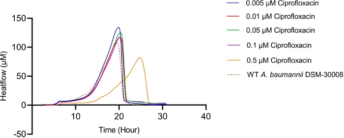
Figure 1A: Please click here to view a larger version of this figure.

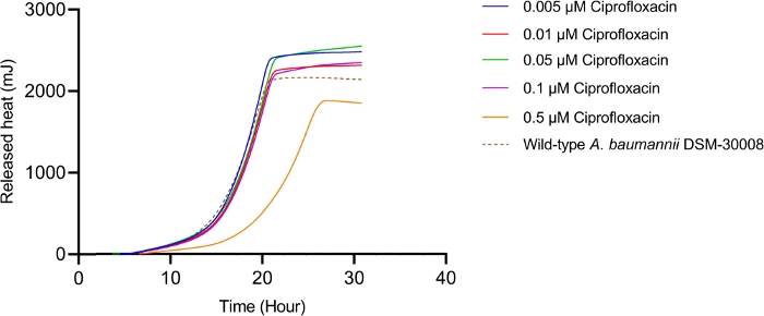
Figure 1B: Please click here to view a larger version of this figure.

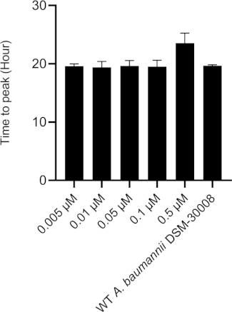
Figure 1C: Please click here to view a larger version of this figure.

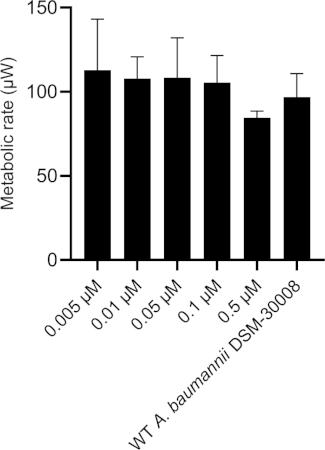
Figure 1D: Effect of ciprofloxacin on A. baumannii DSM-30008 growth and metabolism. (A) Thermograms shown as heat flow (µW) vs. time (h) for wild type (WT) A. baumannii DSM-30008, non-treated and exposed to ciprofloxacin. (B) Cumulative heat (mJ) vs. time (h). (C) Time to peak (h) with error bars (standard deviation). (D) Metabolic rate (µW) with error bars (standard deviation). Please click here to view a larger version of this figure.

In the case of tetracycline, we did not observe significant changes in the thermograms for all concentrations tested until late exponential phase starting after 8 hours (see Figure 2A). Nevertheless, major changes are observed in stationary phase heat emission, where the second peak of heat flow is significantly lowered for A. baumannii treated with 5 µM and 10 µM tetracycline. Lower concentrations had an effect as well, which was however less pronounced. This effect also causes a prolongation in time to peak as displayed in Figure 2C. The cumulative released heat curves (Figure 2B) show that non-treated and treated cells do not display significant differences in the overall curve shape but by tendency, the slope of the curves declines at higher concentrations of tetracycline. This also translates into quantified metabolic rates displayed in Figure 2D, where a concentration-dependent effect, (i.e., decrease of metabolic rate at increasing antibiotic concentrations) is observed. These findings support the fact that tetracycline has a bacteriostatic effect.

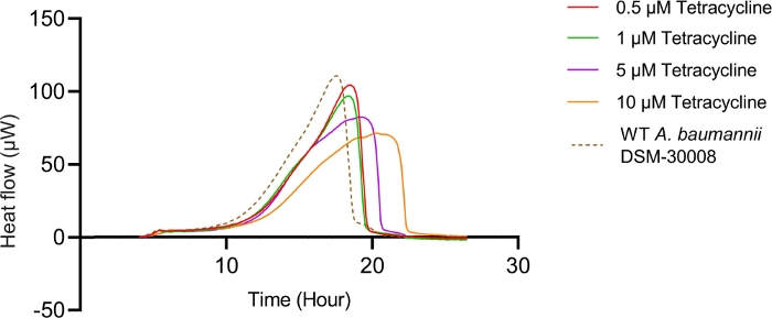
Figure 2A: Please click here to view a larger version of this figure.

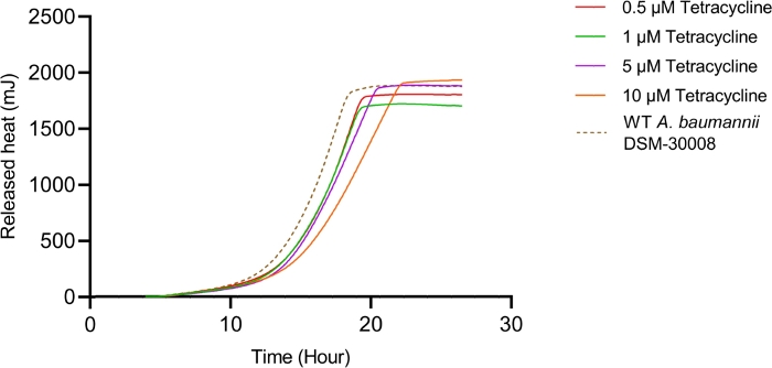
Figure 2B: Please click here to view a larger version of this figure.

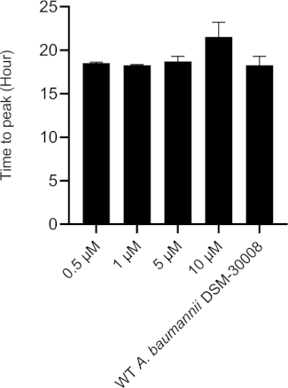
Figure 2C: Please click here to view a larger version of this figure.

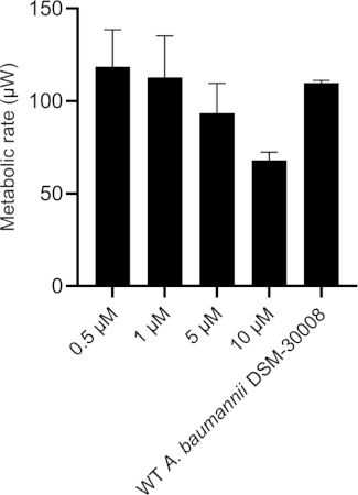
Figure 2D: Effect of tetracycline on A. baumannii DSM-30008 growth and metabolism. (A) Thermograms shown as heat flow (µW) vs. time (h) for wild type (WT) A. baumannii DSM-30008, non-treated and exposed to tetracycline. (B) Cumulative heat (mJ) vs. time (h). (C) Time to peak (h) with error bars (standard deviation). (D) Metabolic rate (µW) with error bars (standard deviation). Please click here to view a larger version of this figure.

Even more pronounced effects can be observed when treating A. baumannii with the protein synthesis inhibitor chloramphenicol that targets the 50S ribosomal subunit. Exposure to increasing concentrations of chloramphenicol leads to prolongation of the lag phase and significant changes of the metabolic activity in the stationary phase (Figure 3A and Figure 3B). No change in metabolic rate is observed for the lowest tested concentration and the highest test concentration chosen (50 µM) prevents most energy release of the sample. Looking at the intermediate test concentrations (5 µM and 10 µM), the time to peak is significantly increased by approximately 8-9 hours (Figure 3C). Simultaneously, the metabolic rate of treated cells is significantly reduced, with 50 µM being lethal (Figure 3D). Overall, the changes observed at concentrations up to 10 µM chloramphenicol are consistent with a bacteriostatic effect of this antibiotic class.

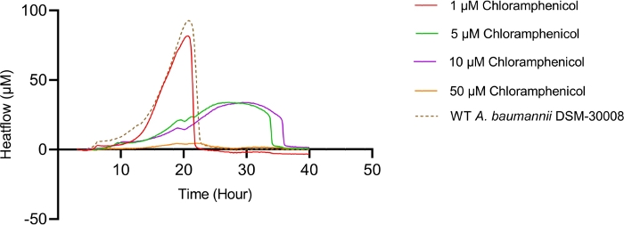
Figure 3A: Please click here to view a larger version of this figure.

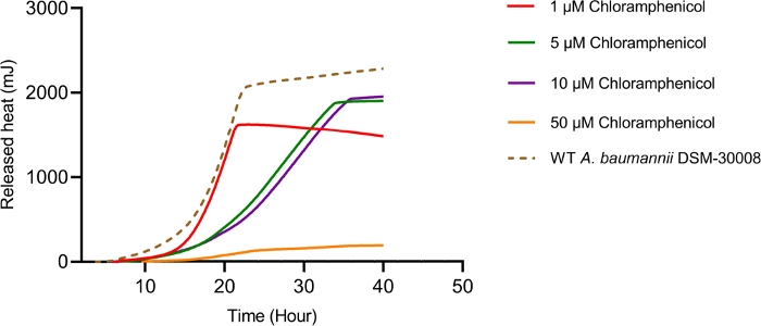
Figure 3B: Please click here to view a larger version of this figure.

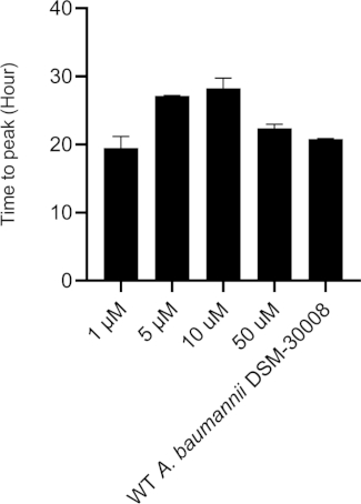
Figure 3C: Please click here to view a larger version of this figure.

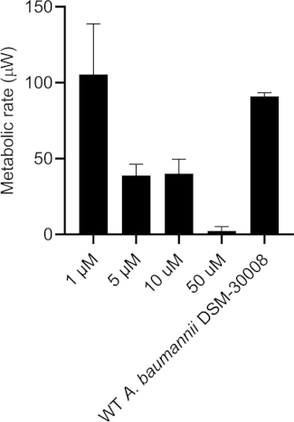
Figure 3D: Effect of chloramphenicol on A. baumannii DSM-30008 growth and metabolism. (A) Thermograms shown as heat flow (µW) vs. time (h) for wild type (WT) A. baumannii DSM-30008, non-treated and exposed to chloramphenicol. (B) Cumulative heat (mJ) vs. time (h). (C) Time to peak (h) with error bars (standard deviation). (D) Metabolic rate (µW) with error bars (standard deviation). Please click here to view a larger version of this figure.

Rifampicin treatment in the selected concentration range has a dramatic effect on the thermograms of A. baumannii DSM-30008 related to the lag phase duration and effects on growth until the late stationary phase (Figure 4A). A significant reduction of heat emission can be seen in Figure 4B that goes along with a decrease in metabolic activity. Figure 4C and Figure 4D illustrate the influence of the prolongation of the lag phase and changes of the metabolic activity in the stationary phase. Figure 4C shows a definite increase in time to peak for all concentrations used. Figure 4D illustrates the decrease in the metabolic rate caused by the decrease in slope for all concentrations that is usually ascribed to a bactericidal effect. Due to antibiotic-induced killing of bacterial cells, the metabolic activity is expected to be lower due to a smaller number of active bacteria present. The data collected are in agreement with the fact that rifampicin can act bactericidal and bacteriostatic, and the data presented here support mainly bactericidal effects of the chosen concentrations.

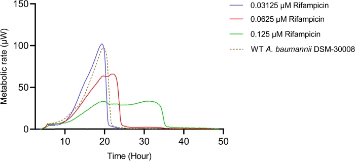
Figure 4A: Please click here to view a larger version of this figure.

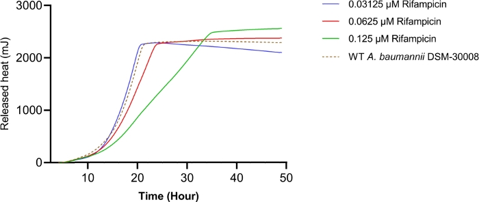
Figure 4B: Please click here to view a larger version of this figure.

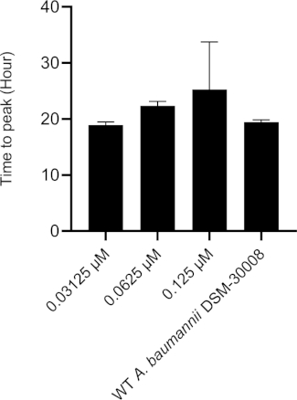
Figure 4C: Please click here to view a larger version of this figure.

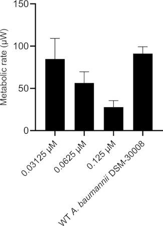
Figure 4D: Effect of rifampicin on A. baumannii DSM-30008 growth and metabolism. (A) Thermograms shown as heat flow (µW) vs. time (h) for wild type (WT) A. baumannii DSM-30008, non-treated and exposed to rifampicin. (B) Cumulative heat (mJ) vs. time (h). (C) Time to peak (h) with error bars (standard deviation). (D) Metabolic rate (µW) with error bars (standard deviation). Please click here to view a larger version of this figure.

The lowest selected test concentration of the natural product antibiotic (0.25 µM) has no or only marginal effects on the thermogram of A. baumannii DSM-30008. However, other tested concentrations exhibit some effect on lag phase duration, and affect the growth until the late stationary phase (Figure 5A). The most obvious effect is the significant reduction of heat emission in the stationary phase. Data displayed in Figure 5B clearly show that released energy is significantly decreased for all effective concentrations and the slope is decreased as well. These effects translate into a decrease of time to peak (Figure 5C) and more importantly, a significant and clearly dose-dependent decrease in metabolic rate is observed (Figure 5D). The investigation of the new myxobacterial natural product revealed a combined bacteriostatic and bactericidal effect.

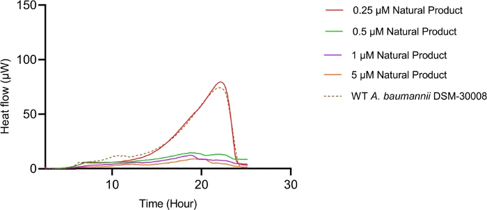
Figure 5A: Please click here to view a larger version of this figure.

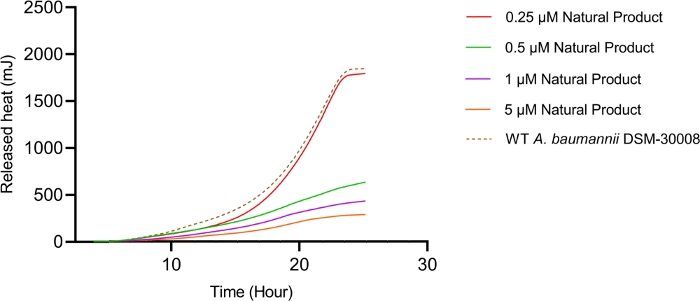
Figure 5B: Please click here to view a larger version of this figure.

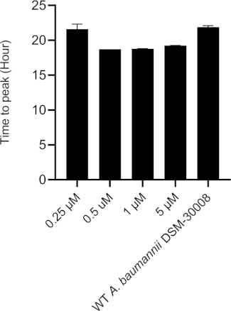
Figure 5C: Please click here to view a larger version of this figure.

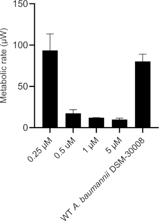
Figure 5D: Effect of a new antibacterial natural product on A. baumannii DSM-30008 growth and metabolism. (A) Thermograms shown as heat flow (µW) vs. time (h) for wild type (WT) A. baumannii DSM-30008, non-treated and exposed to the natural product. (B) Cumulative heat (mJ) vs. time (h). (C) Time to peak (h) with error bars (standard deviation). (D) Metabolic rate (µW) with error bars (standard deviation). Please click here to view a larger version of this figure.

Supplemental Figure 1: Selecting a new experiment in the software interface. In a red square the step to select a new experiment is depicted. Please click here to download this figure.

Supplemental Figure 2: Naming a new experiment in the software interface. In a red square the step to name and confirm the new experiment is depicted. Please click here to download this figure.

Supplemental Figure 3: Starting a new experiment in the software interface. In a red square the step to start a new experiment is depicted. Please click here to download this figure.

Supplemental Figure 4: Well selection and reaction start in software interface. All reaction wells are selected (wells colored in deep blue color, button Select all depicted in a red square) and reaction start is selected (depicted in a red square). Please click here to download this figure.

Supplemental Figure 5: Correct loading of cup holder. Reference wells are selected (deep blue color, red square) and thermograms are displayed in a popup window. When the loading is performed correctly, we observe a steep decline in heat emission signal detected that must reach a plateau phase and remain in this phase for approximately 2-3 min, afterwards the signal returns to the starting point. When this is observed the loading of the cup holder is correct. Please click here to download this figure.

Supplemental Figure 6: End of experiment. In red, the Stop button in the experiment is depicted. Please click here to download this figure.

Supplemental Figure 7: Confirmation of the end of experiment. In red, the Yes button to confirm the end of running experiment is depicted. Please click here to download this figure.

Supplemental Figure 8: Saving the experiment file. A popup window with save file options is shown and in red the button Save is depicted. Please click here to download this figure.

Supplemental Figure 9: Software interface. Please click here to download this figure.

Supplemental Figure 10: Accessing saved experiments. In red the button Open experiment to access saved experiments is depicted. Please click here to download this figure.

Supplemental Figure 11: Opening of selected experiment file. In red the button Open is depicted. Please click here to download this figure.

Supplemental Figure 12: Default wells view. All experimental well and corresponding thermograms are visible. Please click here to download this figure.

Supplemental Figure 13: Selecting wells for analysis. In red the button Select all is depicted. Please click here to download this figure.

Supplemental Figure 14: Defining the baseline. In red the button Define baseline is depicted. Please click here to download this figure.

Supplemental Figure 15: Selecting the baseline signal. Minimum of 30 min of signal in the lag phase is selected (red box). Please click here to download this figure.

Supplemental Figure 16: Saving changes to the experimental file. In red the button Save is depicted. Please click here to download this figure.

Supplemental Figure 17: Web based Calorimetry analysis application. The online software interface and file upload pathway is shown. Please click here to download this figure.

Supplemental Figure 18: Upload of selected experimental file. In red the button Open is depicted. Please click here to download this figure.

Supplemental Figure 19: Analysis of the thermograms. Metabolic parameters calculated for each experimental well are depicted in red. Please click here to download this figure.

Supplemental Figure 20: Fitting the experimental data to theoretical growth models. Heat flow data is fitted either to a Gompertz or a Richard´s growth model. Please click here to download this figure.

Supplemental Figure 21: Exporting the measurements. In red the buttons Download Measures and Save are depicted. Please click here to download this figure.

Discussion

Isothermal microcalorimetry measures energy emitted from a specimen over time and this energy release is a result of all biological, physical and (bio-)chemical processes. The measured heat flow can be exploited to evaluate or determine antibacterial effects of substances as it enables continuous real-time monitoring of metabolic activity.

In order to obtain reliable data for analysis, correct starting colony-forming units (CFU) need to be determined individually for each species or strain used. In case the CFU count is too low, this leads to a prolonged lag phase as it takes longer for the system to reach a critical amount of biomass producing enough heat to be detected. In case the CFU count is too high the lag phase will be very short, and the amount of heat produced can cause heat transfer to neighboring sensor cells (reference and experimental wells) and cause distortions of the thermograms. High numbers of CFU will also lead to a faster oxygen depletion and switch to anaerobic conditions. It also has to be taken into account that during the first 30 minutes of the experiment, when the system is equilibrating, data collection is not possible and the actual recording of effects is delayed. In addition, incorrect CFU determination leads to false MIC determination, ultimately affecting the experiment and the changes observed²⁵. Another critical point is the correct determination of the baseline. Usually, the baseline signal is selected during the lag phase when the heat flow signal is zero and ideally, the time range for baseline definition is >30 min. However, this is not always possible as the time that the bacteria requires to reach the heat signal detection limit differs between strains and species. Some species or strains require more than 30 minutes to reach the heat signal detection limit while other strains or species reach it within the first 30 minutes. In that case, it is possible to select the baseline signal at the end of the experiment when all the heat signals have dropped back to zero and remain stable. Alternatively, baselines from other experiments with the same bacterial strain can be used, which is however not recommended.

The system allows for some flexibility in terms of design and optimization of experiments and troubleshooting. Volumes used are in the range of 100-300 µL when using plastic inserts and 100-600 µL when using titanium cups without the plastic inserts. The recommended working volume by the manufacturer is 120 µL. The use of different volumes in setting up a new experimental series, and while finding optimal conditions for measurements, has an impact mainly on two parameters. By using lower volumes, the amount of required test compound can be decreased, which is particularly important for compounds, which are available only in small amounts. In addition, the used volume directly impacts oxygen availability during the measurement with lower volumes increasing the amount of available oxygen required for bacterial growth. Oxygen depletion is one of the main factors contributing to the maximum possible duration of the experiment. Importantly, it is possible to use solid media, not only liquid media. This is especially important for slow-growing microorganisms as growth on the interface between solid and gas phase enables better oxygen access⁹.

IMC is a useful analytic tool to discover unknown processes with applications in physics, chemistry and biology. The method measures the heat exchange within a closed system and analysis of the recorded heat exchange provides additional information that cannot always be obtained with standard methods. In microbiology and antibiotics research, one of the biggest advantages of IMC is its ability to distinguish between live, dead and persister or dormant cells, which is not possible using standard turbidity methods¹¹. In addition, IMC is highly sensitive and it can detect heat emission from as few as 10⁴-10⁵ cells⁹. Another advantage is that the experimental setup is fast and easy, and it allows for continuous, real-time tracking with minimal to no user interference. Further, IMC is non-destructive, which enables further analysis of samples. Data analysis allows for decoupling of biomass formation until late exponential or early stationary phase and metabolic activity in stationary phase.

Besides the novel and exciting application features mentioned above, there are also drawbacks to this method. The major limitation is that IMC instruments measure the total heat produced and released within a specific system, which also include non-specific signals. This highlights the importance of experimental planning with appropriate controls to be able to assess the heat signal changes that are measured by recording heat flow^9,20.

In our hands, IMC is an important tool to study antibacterial effects of new natural products and to determine effective concentration ranges. Apart from differentiating bacteriostatic and bactericidal effects, it could be used in future as part of target identification studies and MoA determination. This can be done by comparing thermograms of different antibiotic classes to thermograms of new active compounds as displayed here. However, it still has to be investigated whether certain quantifiable parameters that can be extracted from the measured data are sufficient for such comparisons or if it will be necessary to work on algorithms giving fingerprints based on full thermograms. Another possible application in the field of antibiotic research is the comparison of wildtype to resistant clones, coupled with whole genome sequencing, which can help elucidating the mode-of-resistance (MoR) of new antibacterials. Because of the static nature of the method, investigation of efficacy of new agents on either biofilm formation or on already established biofilms could lead to better understanding of the biological process and the effect of selected agents on microbes in different stages of dormancy. IMC records total energy released in the form of heat making it a suitable method to investigate also sub-inhibitory effects of active substances that might be coupled to transcriptomics. This method can also be used in clinical settings to detect contamination of samples or for the determination of antibiograms helping to rapidly decide on definite treatment of the patients¹¹.

Materials

List of materials used in this article

Name	Company	Catalog Number	Comments
Acinetobacter baumannii	DSMZ	DSM-30008	reference strain used in this study
calPlate	Symcel	1220093	48-well plate for titanium cups to be inserted
calScreener	Symcel	1200001	isothermal microcalorimetry instrument
calView software	Symcel		collection and analysis software
calWell	Symcel	1901004	micro-bio grade (non-active) 48-well plate with plastic inserts which are inserted into the titanium cups
CASO agar	Carl Roth	X937.1	isolation and cultivation of microorganisms
Chloroamphenicol	Sigma-Aldrich	C0378	antibiotic
Ciprofloxacin	Sigma-Aldrich	17850	antibiotic
Cuvettes	Brand	759015	1.5 mL cuvettes
Disposable inoculation loops	Sarsted	86.1562.050	10 µL inoculation loops
Dimethylsulfoxid (DMSO)	Thermo Fisher Scientific	85190
Eppendorf tubes	Eppendorf	30120086	1.5 mL eppendorf safe-lock tubes
Ethanol	Thermo Fisher Scientific	10428671
Falcon Tubes	Sarsted	62.554.502	15 mL falcon tubes
Hydrochloride (HCL)	Thermo Fisher Scientific	10316380
Methanol	Thermo Fisher Scientific	A412-500
Mueller Hinton Broth	Sigma-Aldrich	70192	liquid medium for antibiotic susceptibility studies
Mueller Hinton Broth II cation adjusted media	Sigma-Aldrich	90922	Mueller Hinton Broth cation-adjusted to 1.25 mM CaCl2, 0.8 mM MgCl2
Petri dishes	LABSOLUTE	7696404
Pipette 100 - 1000 µL	Brand	705880
Pipette 2 - 20 µL	Brand	705872
Pipette 20 - 200 µL	Brand	705878
Pipette tips 100 - 1000 L	Brand	732032
Pipette tips 2 - 200 µL	Brand	732028
Polymyxin B sulfate	Sigma-Aldrich	P0972	antibiotic
Rifampicin	Sigma-Aldrich	R3501	antibiotic
Serological pipette	Thermo Fisher Scientific	170356N	10 mL Nunc serological pipette
Spectrophotometer	Eppendorf AG	6135 000.017
Sterile filters	Minisart	16534----------K	0.2 µm pore size sterile filters
Syringe 50 mL	NORM-JECT	22778
Tetracycline	Sigma-Aldrich	87128	antibiotic
Titanium cups	Symcel	1220089	inserted in 48-well titanium calPlate
Titanium lids	Symcel	1220091	screwed and tightend to the titanium cups
Trimethroprim	Sigma-Aldrich	T7883	antibiotic
Tweezers	Symcel	1900602

References

- World Health Organization (WHO). Antibiotic resistance. World Health Organization (WHO). , Available from: https://www.who.int/news-room/fact-sheets/detail/antibiotic-resistance (2018).
- Herrmann, J., Abou Fayad, A., Müller, R. Natural products from myxobacteria: novel metabolites and bioactivities. Natural Product Reports. 34 (2), 135-160 (2017).
- Cassar, S., et al. Use of Zebrafish in Drug Discovery Toxicology. Chemical Research in Toxicology. 33 (1), 95-118 (2020).
- Bhusnure, O. G., et al. Drug Target Screening and its Validation by Zebrafish as a Novel Tool. Pharmaceutica Analytica Acta. 6 (10), 426(2015).
- Kraus, J., Tobin, G., Development, Discovery, Deveopment, and Regulation of Natural Products. Using Old Solutions to New Problems - Natural Drug Discovery in the 21st Century. Kulka, M. , InTech. Rijeka, HR. 4-36 (2013).
- Tabassum, N., Tai, H., Jung, D., Williams, D. R. Fishing for Nature's Hits: Establishment of the Zebrafish as a Model for Screening Antidiabetic Natural Products. Evidence-Based Complementary and Alternative Medicine. 2015 (1), 287847(2015).
- Antimicrobial Development. Symcel. , Available from: https://symcel.com/applications/microbiology/antimicrobials-development (2019).
- Robador, A., LaRowe, D. E., Finkel, S. E., Amend, J. P., Nealson, K. H. Changes in Microbial Energy Metabolism Measured by Nanocalorimetry during Growth Phase Transitions. Frontiers in Microbiology. 2018 (9), 109(2018).
- Braissant, O., Wirz, D., Göpfert, B., Daniels, A. U. Use of isothermal microcalorimetry to monitor microbial activities. FEMS Microbiology Letter. 303 (1), 1-8 (2010).
- Braissant, O., et al. Isothermal microcalorimetry accurately detects bacteria, tumorous microtissues, and parasitic worms in a label-free well-plate assay. Biotechnology Journal. 10 (3), 460-468 (2015).
- Butini, M. E., Abbandonato, G., Di Rienzo, C., Trampuz, J., Di Luca, M. Isothermal microcalorimetry detects the presence of persister cells in a Staphylococcus aureus biofilm after vancomycin treatment. Frontiers in Microbiology. 25 (10), 332(2019).
- Tellapragda, C., et al. Isothermal microcalorimetry minimal inhibitory concentration testing in extensively drug resistant Gram-negative bacilli - A multicenter study. Clinical Microbiology and Infection. , (2020).
- Abdillahi, S., et al. Collagen VI Contains Multiple Host Defense Peptides with Potent In Vivo Activity. The Journal of Immunology. 201 (3), 1007-1020 (2018).
- Astasov-Frauenhoffer, M., et al. Exopolysaccharides regulate calcium flow in cariogenic biofilms. PLoS ONE. 12 (10), 1-14 (2017).
- Gros, S., et al. Personalized Treatment Response Assessment for Rare Childhood Tumors Using Microcalorimetry-Exemplified by Use of Carbonic Anhydrase IX and Aquaporin 1 Inhibitors. International Journal of Molecular Sciences. 20 (20), 4984(2019).
- Kriszt, R., et al. Optical visualisation of thermogenesis in stimulated single-cell brown adipocytes. Scientific Reports. 7 (1), 1-14 (2017).
- Wadsö, I., et al. A well-plate format isothermal multi-channel microcalorimeter for monitoring the activity of living cells and tissues. Thermochimica Acta. 652 (1), 141-149 (2017).
- von Ah, U., Wirz, D., Daniels, A. U. Isothermal micro calorimetry - a new method for MIC determinations: results for 12 antibiotics and reference strains of E. coli and S. aureus. BMC Microbiology. 9 (106), (2009).
- Howell, M., Wirz, D., Daniels, A. U., Braissant, O. Application of a Microcalorimetric Method for Determining Drug Susceptibility in Mycobacterium Species. Journal of Clinical Microbiology. 50 (1), (2012).
- Wadsö, I. Isothermal Microcalorimetry: Current problems and prospects. Journal of Thermal Analysis and Calorimetry. 64 (2001), 75-84 (2001).
- LeBel, M. Ciprofloxacin: chemistry, mechanism of action, resistance, antimicrobial spectrum, pharmacokinetics, clinical trials, and adverse reactions. Pharmacotherapy. 8 (1), 3-33 (1988).
- Chopra, I., Roberts, M. Tetracycline antibiotics: mode of action, applications, molecular biology, and epidemiology of bacterial resistance. Microbiology and Molecular Biology Reviews. 65 (2), 232-260 (2001).
- Allison, J. L., et al. Mode of action of chloramphenicol. VII. Growth and multiplication of Escherichia coli in the presence of chloramphenicol. Journal of Bacteriology. 83 (3), 609-615 (1962).
- Wehrli, W. Rifampin: mechanisms of action and resistance. Reviews of Infectious Diseases. 5, Suppl 3 407-411 (1983).
- Hancock, R. E. W., et al. Agar and broth methods to determine the minimal inhibitory concentration (MIC) of antimicrobial substances. Nature Protocols. 3 (2), 163-175 (2008).
Reprints and Permissions