Development and Testing of Species-specific Quantitative PCR Assays for Environmental DNA Applications

Summary

Environmental DNA assays require rigorous design, testing, optimization and validation before the collection of field data can begin. Here, we present a protocol to take users through each step of designing a species-specific, probe-based qPCR assay for the detection and quantification of a target species DNA from environmental samples.

Abstract

New, non-invasive methods for detecting and monitoring species presence are being developed to aid in fisheries and wildlife conservation management. The use of environmental DNA (eDNA) samples for detecting macrobiota is one such group of methods that is rapidly becoming popular and being implemented in national management programs. Here we focus on the development of species-specific targeted assays for probe-based quantitative PCR (qPCR) applications. Using probe-based qPCR offers greater specificity than is possible with primers alone. Furthermore, the ability to quantify the amount of DNA in a sample can be useful in our understanding of the ecology of eDNA and the interpretation of eDNA detection patterns in the field. Careful consideration is needed in the development and testing of these assays to ensure the sensitivity and specificity of detecting the target species from an environmental sample. In this protocol we will delineate the steps needed to design and test probe-based assays for the detection of a target species; including creation of sequence databases, assay design, assay selection and optimization, testing assay performance, and field validation. Following these steps will help achieve an efficient, sensitive, and specific assay that can be used with confidence. We demonstrate this process with our assay designed for populations of the mucket (Actinonaias ligamentina), a freshwater mussel species found in the Clinch River, USA.

Introduction

Researchers and managers are increasingly becoming interested in the use of environmental DNA assays for species detection. For three decades, quantitative or real time PCR (qPCR/rtPCR) has been used in numerous fields for the sequence-specific detection and quantification of nucleic acids^1,2. Within the relatively new field of eDNA research, use of these assays with a standard curve for quantification of copies of target DNA per volume or weight of eDNA sample has now become routine practice. Mitochondrial DNA sequences are generally targeted in eDNA assays because the mitochondrial genome is present in thousands of copies per cell, but assays for nuclear DNA or RNA sequences are also possible. It is vital to understand that published assays for eDNA samples are not always equal in performance. An assay’s reliability in detecting only the DNA of a target species (i.e., specificity) and detection of low quantities of target DNA (i.e., sensitivity) may vary considerably due to differences in how the assay was designed, selected, optimized and tested. Reporting quantitative measures of assay performance has been previously largely overlooked, but recently standards to improve transparency in assay development are emerging^3,4,5,6,7,8.

Optimization and reporting of assay performance aids in study design and interpretation of eDNA survey results. Assays that cross-react with non-target species DNA could lead to false positive detections, while assays with poor sensitivity may fail to detect the target species DNA even when it is present in the sample (false negatives). An understanding of assay sensitivity and selectivity will help inform the sampling effort needed to detect rare species. Because there are many natural sources of variation in eDNA, studies must limit controllable sources of variation as much as possible, including fully optimizing and characterizing the eDNA assay³.

Conditions that directly affect an assay’s specificity or sensitivity will change the assay’s performance. This can occur under different laboratory conditions (i.e., different reagents, users, machines, etc.). Therefore, this protocol should be revisited when applying an assay under new conditions. Even assays well-characterized in the literature should be tested and optimized when adopted by a new laboratory or when using different reagents (e.g., master-mix solution)^5,9. Assay specificity may change when applied to a different geographic region, because the assay is being applied to samples from a new biotic community that may include non-target species that the assay has not been tested against, and genetic variation in the target species may occur. Again, the assay should be re-assessed when used in a new location. Field conditions differ from laboratory conditions because in the field PCR inhibitors are more likely to be present in samples. PCR inhibitors directly affect the amplification reaction and thus affect assay performance. For this reason, an internal positive control is required when developing an eDNA assay.

Finally, environmental conditions in the field can affect the target species' DNA molecules and their capture through DNA degradation, transport and retention. Furthermore, different protocols for DNA collection and extraction vary in their efficiency and ability to retain DNA. However, it is important to note that these processes affect the detectability of eDNA but not a molecular assays’ performance. Thus, detectability of DNA from the target species in field samples is a function of both the technical performance of the qPCR assay as well as field conditions and collection, storage, and extraction protocols. When using a well characterized and highly performing assay, users can feel confident in the assay’s capabilities; allowing researchers to now focus on understanding the external assay factors (i.e., environmental variables, differences in capture or extraction protocols) affecting eDNA detection.

Here we focus specifically on assay technical performance through rigorous design and optimization. We demonstrate the protocol using a probe-based assay developed for the detection of a freshwater mussel, the mucket (Actinonaias ligamentina), from water sampled in the Clinch River, USA. Recently Thalinger et al. (2020) presented guidelines for validation of targeted eDNA assays. Assay design following our protocol will bring an assay to Thalinger et al.’s level 4 plus an additional step towards level 5⁶. At this point an assay’s technical performance will be optimized and it will be ready for regular use in laboratory and field applications. Further use of the assay in laboratory, mesocosm, and field experiments can then address questions regarding eDNA detection and factors influencing detectability, the final steps for level 5 validation⁶.

Protocol

1. Generation of a sequence database of mitochondrial DNA sequences from target and non-target species of interest

1. Define the question, targets and system being addressed. Identify the target species for eDNA detection. Identify the geographic system in which the assay will be used. Make a list of species of interest, including the target species, sympatric (co-occurring) species within the same taxa (usually order or family level), and closely related allopatric species, those that may not be in the same geographic location as the target (Figure 1).
   NOTE: Here, the Clinch River populations of the species A. ligamentina were targeted.
2. Search and download sequences from multiple gene regions for species on the list from Step 1. Sequence databases such as NCBI (National Center for Biotechnology Information), BOLD (Barcode of Life Database), EMBL (European Molecular Biology Laboratory) and DDBJ (DNA Data Bank of Japan) can be used. NCBI, EMBL and DDBJ all share sequence information.
   1. Using NCBI’s Nucleotide Database, search for the target organism (e.g., Actinonaias ligamentina) and gene region (e.g., cytochrome c oxidase I (COI) or NADH-dehydrogenase 1 (ND1); Example search string: Actinonaias ligamentina AND ND1)
   2. Next, select all sequences that match the specifications and select Send to. Choose Complete record, File and download format as either GenBank or FASTA and then Create File. These sequences are now saved to the computer.
   3. Repeat these steps for all the species on the list defined in Step 1. Keep sequences for each gene region in a separate file as these will be analyzed separately.
      1. Download all relevant sequences (or a large, representative proportion of sequences) for the target species identified in Step 1. Include geographic variants if possible.
      2. Repeat the search and download sequences for related and sympatric non-target species of the same taxonomic group that were identified in Step 1 (e.g., if the target species is the mucket (A. ligamentina) download sequences for all other freshwater mussel species in the Family Unionidae that occur in the system of interest).
      3. Repeat the search and download for closely related but allopatric (geographically separate) species listed in Step 1.1.
         NOTE: Not all species (targets and non-targets) will be available in the public databases. Increase the local reference database by amplifying and sequencing taxonomically verified specimens of species of interest in-house. If working with a species that has high within-species genetic diversity or working in a geographically large area where geographic variants may be expected, gather sequences from across the range.

2. Assay design

1. Align sequences from each gene region separately using alignment software that can be found in various genetic sequence editing and bioinformatic programs. Do this alignment for each of the different gene regions.
   1. For instance, using Geneious Prime software (https://www.geneious.com) import the downloaded sequence files into the program.
   2. Create separate folders for each gene region.
   3. Within a folder that contains sequences from one gene region, select all the sequences.
   4. Use the Multiple alignment tool to create a nucleotide alignment of the selected sequences. There may be several options for the type of alignment, using the Geneious or MUSCLE alignments and default parameters works well.
2. Choose promising regions for assay design through the visualization of aligned sequence data. A region that has a lot of sequence data available for the species of interest, is highly divergent among species, and shows low within-species variation is a good candidate. This will increase the likelihood that primers and probes designed will be able to discriminate the target from non-target species, while also ensuring intraspecific variants will amplify with the assay.
3. Design of assay primers and probe.
   1. Use qPCR assay design software and follow instructions. IDT’s PrimerQuest Tool (https://www.idtdna.com/) to design 5 sets of qPCR assays was used here.
   2. Paste the sequence selected in step 2.2 into the Sequence entry box. If the alignment created spaces, delete those from the sequence.
   3. Select qPCR 2 Primers + Probe in the Choose Your Design option.
   4. Download the recommended assays.
   5. Copy the sequences from the forward primer of the first assay, and search for this primer sequence in the alignment created in step 2.1.4. If using Geneious Prime, use the Annotate and Predict tool to add the primer region to the alignment. Do this for all the primer and probe combinations (Figure 2).
   6. Inspect these regions of the alignment for variation within the target species as well as within the co-occurring species.
      1. If there is intraspecific genetic variation, search for assays where the primers and probe do not fall within these regions.
      2. To prevent non-target species amplification, search for mismatches with non-target species. Choose assays with the most mismatches for further validation. Currier et al. (2018) suggest choosing sets with at least two of the three regions (the two primers, or a primer and a probe) having at least two mismatches with all the non-target species. However, keep in mind that mismatches at the probe contribute less to specificity¹⁰.
         NOTE: Differences within 3 base pairs of the 3’ end of each primer increase specificity better than differences at the 5’ end of the primers¹⁰.
   7. Consider the following important parameters in assay design.
      1. Determine the melting and annealing temperatures of the primers and probe. Ideally the melting temperature (Tm) of primers should be between 60-64 °C and within 2 °C of each other, and the Tm of the probe should be 6-8 degrees higher than the Tm of the primers. Set the annealing temperature (Ta) of the qPCR reaction 5 °C below the melting temperature, around 55-60 °C¹¹.
      2. Examine the GC content. Choose between 35 – 65% GC content, and avoid regions with 4 or more consecutive Gs. Having 1 or 2 Gs or Cs in the 5 last bases of the 3’ end of the primer (GC clamp) might increase specificity as it would help the primer to make a stronger bond¹².
      3. Search for hairpin and dimer structures. Test primers and probe for predicted hairpin structures and dimers using an oligonucleotide analyzing program (e.g., OligoAnalyzer -IDT¹³; OligoCalculator¹⁴). These structures can cause non-target amplification and lower efficiency. Avoid assays which are predicted to form these structures.
      4. Determine the primer length. Aim for primers between 18-25 bases in length and probe length between 20 –25 bases. Longer primers and probes may have lower amplification efficiency.
      5. Determine the amplicon length. It should be between approximately 100 and 250 base pairs. This range is generally short enough for high PCR efficiency, but long enough for ease of verification by Sanger sequencing^4,15.
      6. Design probes. Make sure the probes do not have a G base at the 5’ end, because it could dampen the signal from green and yellow dyes¹¹. We designed double quenched probes, with IDT 3IABkFQ and ZEN quenchers and FAM or HEX fluorophores.
         NOTE: Determine the MGB probes: TaqMan MGB (minor groove binder) probes are often used for eDNA studies. However, because these probes are very short, they can bind to non-targets even with a 2 or 3 base pair mismatch¹⁰.
      7. Determine the probe Tm. Melting temperature of the probe should be 6-8°C higher than the primers. Lower temperatures decrease the binding success of the probe.
      8. Determine the probe length and location. The probe should be between 20 and 25 bp in length and ideally located close to the primer binding site on the same strand without overlapping it.

3. Assay screening and optimization

1. In silico assay development and testing. Before ordering primer-probe sets, assess specificity (potential non-target amplification) by testing primer amplification in silico.
   1. Test primers through NCBI’s Primer-Blast¹⁶ or similar programs that can identify potential non-targets in the NCBI nt/nr database that might amplify with the assay. If using Primer-Blast paste primers on the Use my own primer box under Primer parameters. In the Primer Pair Specificity Checking Parameters options, select nr as the Database and type the Order of the organism of interest (e.g., “Unionida” or “Unionoida”) in the Organism box.
   2. Continue to assess primer/probe sets visually on aligned sequence data.
      1. In order to assess primers and probes at the same time in silico, create a text string of the forward primer, 12 N’s, the probe, 12 N’s, and the reverse complement of the reverse primer. If the probe sequence is within 12 base pairs of one of the primers, use the number of N’s corresponding to the number of base pairs between the primer and probe.
      2. Use NCBI’s Nucleotide Blast search (Blastn) to search against the nr database¹⁷. Use the Taxonomy tab to look for non-target species with few mismatches; these should be tested in the laboratory during assay optimization.
         NOTE: In silico testing helps rule out non-specific assays, but potentially specific assays must be tested empirically (in vitro), as not all species have sequences in the genetic databases and primer and probes can still bind to non-targets even if deemed unlikely by the software.
2. Choose three to five primer/probe combinations to test in the laboratory.
3. Order primers, probes and a synthetic DNA standard as well as additional M13-tailed primers for amplicon sequencing.
   1. Order synthetic oligonucleotide primers and probes from a company that makes oligos. Probes are labelled with a fluorescent dye and a quencher. Different fluorophores should be selected for assays that need to be multiplexed. Check your qPCR instrument for a list of which fluorophores the instrument can detect.
   2. Design and order M13-tailed primers for verification of qPCR detections with Sanger sequencing by adding the M13 Forward (-20) sequence, GTA AAA CGA CGG CCA GT, to the 5’ end of the forward primer, and the M13 Reverse (-27) sequence, CAG GAA ACA GCT ATG AC, to the 5’ end of the reverse primer.
   3. The synthetic DNA standard contains the target sequence (including the primer regions) at a known concentration in copies/µL. Quantify unknown samples based on a curve made by known concentrations of this standard (i.e., the standard curve). Acquire the synthetic standard from the same company that manufactures the primers and probe. Follow manufacturer recommendations for resuspension and storage. Dilute standards in TE buffer with a tRNA carrier using low-retention plasticware to reduce hydrolysis and binding to surfaces.
      NOTE: If the standard curve does not perform well (poor PCR efficiency, see step 3.4.2), try re-suspending the standard in water or Tris-HCl.
   4. Suspend primers and probes in nuclease free water, Tris-HCl, or TE buffer at convenient concentrations for assay use. Generally, dilute working stocks 20-fold in the master mix to achieve the optimized final assay concentration. Store suspended oligos at a constant -20 °C when not in use.
4. In vitro (in the laboratory) assay optimization and testing. Reject assays that have poor efficiency, cross-react with co-occurring species, or have poor sensitivity¹⁸. Include the use of an internal positive control (IPC) during assay development as well as when running actual samples.
   1. First, find the optimal temperature and primer/probe concentration values for the assay. Once these parameters have been optimized for PCR efficiency (Step 3.4.2), cross-reactivity (Step 3.4.3) and sensitivity (Step 3.4.4), proceed to test the assay with a multiplexed IPC (Step 3.4.5).
      1. Test optimum annealing temperature (Ta) for primer and probes using a PCR temperature gradient centered 5° C below the predicted average primer Tm.
      2. Test optimum primer and probe concentrations. Typically, 200 nM, 400 nM, and 800 nM primer concentrations and 75 nM, 125 nM, and 200 nM probe concentrations are tested.
   2. Create a standard curve and determine efficiency and linear range. Test at least six 10-fold dilutions of a synthetic DNA standard containing the target sequence, at approximately 10⁰ copies/reaction to 10⁵ copies/reaction (Figure 3A).
      1. Use the qPCR software to plot the Cq value (threshold for cycle at quantification) of each standard on the y-axis and the log base 10 of the initial standard concentration in copies/reaction on the x-axis. The qPCR software should automatically run a linear regression (Figure 3B).
      2. Calculate the efficiency from the slope of the regression, E = -1 + 10^(-1/slope). For example, if the slope is -3.4, E= -1 + 10^(0.29) = 0.97 or 97%. Also check the r² values which indicate how well the standard replicates fit on the curve. The qPCR software should automatically calculate this as well (Figure 3B). Aim for efficiency values of 100% (±10%) and r² values of ≥0.98^{9,15,19,20,21,22}.
      3. Visually inspect the standard curve for bias, that is, deviations from the regression in a consistent direction or for poor standard curve performance as measured by efficiency and r² values (Figure 3C and 3D).
   3. Specificity: Assess cross-reactivity with non-target species to decrease the chance of false positives. Where eDNA detections may result in costly management decisions, verify positive detections by amplicon sequencing.
      1. Non-targets: Run the assay against genomic DNA extractions of taxonomically verified specimens of related species and of geographically co-occurring species; with highest priority being to test against closely related, co-occurring species. Use similar total DNA concentrations for both target and non-target samples. The concentration chosen should yield amplification from target species samples near the middle of the linear range of the standard curve. Amplification should be observed only with the target species.
      2. If non-target amplification is observed, clean and sequence the product to verify its identity. It is not uncommon to observe contamination from the target species in tissue samples of non-target species, thus all amplifications at this stage should be verified by sequencing. Reamplify cleaned amplicons from specificity tests using the M13 tailed primers and sequence with M13 primers.
         1. In the post-PCR laboratory, transfer the qPCR products to be sequenced to fresh tubes. Remove residual primers and reaction components with a clean-up kit (e.g., MinElute PCR Purification Kit).
         2. Make 1:100 dilutions of the elutions and amplify 1 µL of each for 30 cycles in a 50 µL PCR reaction with the M13 tailed primers and a high-fidelity polymerase (e.g., Phusion High-Fidelity DNA Polymerase).
         3. Run 10 µL of each reaction on a 1% agarose gel to check for a single band of the expected size. If no band is observed, increase the number of cycles or the amount of sample. If multiple bands are observed, gel purify the band of the expected size.
         4. Remove residual primers and reaction components with a clean-up kit as above and measure the DNA concentrations of the elutions.
         5. Set up sequencing reactions with the M13 primers according to the instructions of the sequencing facility.
            NOTE: Never open amplified samples in the qPCR laboratory. Prepare samples for sequencing in a laboratory dedicated to post-PCR samples.
   4. Sensitivity: Sensitivity affects the chance of false negatives, or failures to detect the target species DNA when it is present. Assess the limit of detection (LOD) and limit of quantification (LOQ) for each assay. Finally, include an internal positive control (IPC) to assess PCR inhibition of samples. Multiplex and test this IPC assay with the designed assay to ensure the two assays do not interfere with one another.
      1. LOD: Make six 4-fold serial dilutions of the synthetic DNA standard, with 8-24 replicates per standard dilution (Figure 4). Calculate the lowest initial concentration with 95% detection. LOD and LOQ plots can be generated with an LOD/LOQ calculator R script⁵.
         NOTE: Data below the LOD should not be censored. Because of the specificity of PCR, there is no lower limit for true positives. The LOD is the highest concentration below which false negatives may be expected to occur.
      2. LOQ: From the same dilution series, calculate the lowest initial DNA standard concentration quantifiable with a coefficient of variation (CV) below 35%.
         NOTE: LOD and LOQ should be reported in copies/reaction. When using a validated assay and field samples amplify below the LOQ, results should be reported as % detections rather than eDNA concentrations, because the exact concentration cannot be measured with confidence⁵.
   5. Use an internal positive control (IPC) to test for PCR inhibition. Inhibition can lead to a decrease in sensitivity and false negatives. Test the ability of the IPC assay to be multiplexed with the target assay.
      1. An IPC assay can be multiplexed with the target assay using a probe with a different reporter dye than the target assay. This IPC assay consists of a short synthetic DNA sequence from a species unrelated to the target taxa, incorporated into the qPCR master mix at a low concentration of approximately 10² copies/reaction, along with primer and probes that detect it. This lower concentration is necessary to avoid competition with the target sequence for polymerase and nucleotides²³.
      2. Compare the Cq value of the sample’s IPC template to that of the IPC template in the no template control. In this no template control (NTC), the only DNA input is that of the IPC template. The IPC template in this reaction should amplify as expected. If the IPC template in a sample amplifies at 2 or more cycles different from that of the IPC template in the NTC, the eDNA sample is inhibited. Samples that do show inhibition can be diluted 1:10 and re-tested. If a sample remains inhibited, that sample should be removed from analysis.
5. In situ assay development and testing
   1. In the laboratory: If access to the organism in the laboratory as well as sympatric species is available; take water samples from enclosures with these species, process the samples and test the assay against these eDNA samples. Sequence products as above to verify amplification of the intended target using the M13 tailed primers.
   2. In the field:
      1. Identify sites where the target organism is known to occur and known not to occur. It is preferable to have some measure of abundance at each site where the target species occurs.
      2. Decide what sample volumes and sample collection methods (e.g., filtration, centrifugation, etc.) will be used.
      3. Include a field blank or negative control at each site, this is clean water that has been brought to the field site and then collected and prepared with the same field equipment and protocols used for eDNA sampling²⁴. The purpose of the field blank is to detect contamination of the sampling equipment and field gear brought to the site. Take the field blank before processing field water samples.
      4. Take multiple water samples per site, preferably 3 samples per site.
      5. Back in the laboratory, process and extract samples.
      6. Run the assay using a plate set up similar to Figure 5A and compare eDNA concentration and detection frequency with known site differences in occurrence and abundance. Confirm all detections by sequencing^24,25.
         NOTE: The above would validate an assay through Level 4 of Thalinger et al.'s (2020) scale⁶ (optimization of the assay’s technical performance) and begin to gather data supporting Level 5 assay validation. Level 5 incorporates probability modeling and use of the assay for eDNA ecology studies. We feel this is beyond the scope of basic assay development, but we encourage these applications of laboratory and field vetted assays to improve assay design and data interpretation.

Results

In designing a species-specific qPCR assay for the mucket (A. ligamentina), available sequences of all Unionidae species in the Clinch river were downloaded. Closely related species such as Lampsilis siliquoidea were also included in the reference database even though they are not found in the same river. Not all species in the river system of interest were found in GenBank, so additional species were sequenced in house. Sequences were aligned using Geneious software and Primer Quest (IDT) software was used to design multiple assays. Five sets of primers and probe were added to the alignment for visual assessment (Figure 2). They were then tested in silico using Primer-Blast, after which they were ordered for further testing in vitro. In the laboratory, all assays were tested using DNA extractions of 27 available species to verify specificity. One assay (A.lig.1) successfully amplified only the target species (Table 1; Table 2). This assay moved forward for further testing of assay efficiency, LOD and LOQ. It has an amplicon length of 121 base pairs. Table 3 shows the sequence used for the A. ligamentina synthetic DNA standard. Figure 3A and Figure 3B show the results of a successful assay with good efficiency and r² values. Figure 3C and Figure 3D show an assay whose standard curve has a poor efficiency; this assay was discarded. The LOD and LOQ for the selected assay (A.lig.1) were both found to be 5.00 copies/reaction using the discrete method described in Klymus et al⁵. The IPC that was multiplexed with the assay (Tables 3-6) did not affect the A. ligamentina assay’s standard curve. The IPC we use is a fragment of the mouse HemT transcript. This assay was predesigned by IDT for another application, but we modified its use as an IPC for our lab’s eDNA applications.

A successful qPCR run should meet certain criteria for each measure of performance (i.e., standard curve amplification, genomic DNA positive control, no template control and internal positive control). The target assay standards should have exponential amplification curves. These curves should reach an end point plateau if allowed to run enough cycles. This is indicative of the fluorescent probe being completely consumed during the reaction, and fluorescence levels reaching a maximum limit. Later amplifying standards may not reach a plateau in 40 cycles. The positive controls (genomic DNA and IPC) should have the same pattern. Unknowns may or may not amplify, but amplification in unknowns should also have an exponential pattern and an endpoint plateau (Figure 5).

In a quality qPCR, the standard dilutions amplify at evenly spaced Cq of approximately every 3.3 cycles for each 10-fold difference in concentration. Each replicate of a standard dilution amplifies in a tightly grouped manner having nearly the same Cq (represented by the r² values). All standard dilutions should exhibit amplification (Figure 3A). In a poor qPCR, standards may exhibit non-exponential shape, uneven variation in Cq values between dilutions, not come to an endpoint plateau, or some dilutions may not amplify at all (Figure 3D).

The important parameters for a standard curve are efficiency, r², slope, and y-intercept. Efficiency should fall between 90%-110% with ideal values near 100% and r² values should be above 0.98 with ideal results approaching 1.0^15,22. Slope values should be between -3.2 and -3.5 with ideal results near -3.3²². The y-intercept values should fall between a Cq of 34-41 with ideal results having a Cq of 37.0. The y-intercept is the predicted Cq of a reaction with 1 copy of the target sequence, the smallest unit that can be measured in a single qPCR. Unknowns with Cq’s greater than the y-intercept are likely to be inhibited. Running greater than 40 cycles of PCR may be necessary to detect the target in case of inhibition or an inefficient primer set, however quantification is not possible under these circumstances and additional negative controls without the target sequence, but containing total DNA similar to the unknowns, should be run to rule out amplification from non-specific sources.

The Internal Positive Control (IPC) amplification in unknown samples should be compared to the results of the negative template control IPC, as there is no competition for reagents and no inhibitors are present. Unknowns with an IPC having a Cq of 2 cycles or greater than the average Cq value of the NTC, or that do not amplify should be considered inhibited. If no inhibitors are present in the samples, then all IPC amplification should have a tight grouping in the plot with Cq values near the same as the NTC (Figure 6).

Finally, in situ testing of the assay occurred. Twenty water samples from the Clinch River and three field blank sample were filtered between September 25-26, 2019 within 500 meters from a mussel bed known to have A. ligamentina. Approximately four 1 L samples of water were filtered per sampling location. Location sites included at the bottom of the mussel bed in stream, bottom of the mussel bed near shore, 100 m downstream of the bed in stream, 500 m downstream of the bed in stream and 500 m downstream of the bed near shore (Figure 7). Back in the laboratory, each filter was cut in half and DNA was extracted from only half of a filter. The remaining filter half for each sample was stored in a -80 °C freezer. Samples were then run using the A.lig.1 assay multiplexed with the IPC. Of the 23 samples, five were found to be inhibited. These samples were diluted 1:10 and dilutions were re-run. Nineteen of the 20 field samples amplified using the designed assay. Of these 19 samples, five were above the assay’s LOD and LOQ of 5 copies/reaction; meaning most of the samples had an eDNA detection but at a level where false negative results are likely to occur and that the assay could not confidently quantify the copy number for those 14 samples. Nevertheless, 75 to 100% of the four biological site replicates amplified at each sampling location. Two of the three field blanks were negative, while one field blank did show amplification, emphasizing the importance of clean technique in the field.

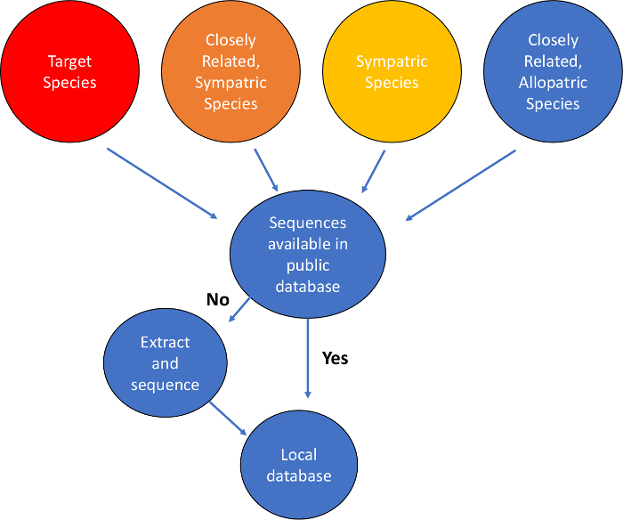
Figure 1: Workflow for mitochondrial DNA sequence database construction.Please click here to view a larger version of this figure.

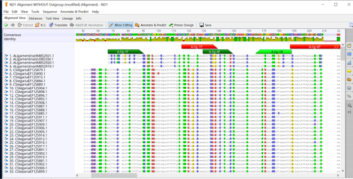
Figure 2: Sequence alignments for Clinch river mussel species with prospective primers and probes for the Actinonaias ligamentina ND1 assay. Forward primers in dark green, probe in red and reverse primer in light green. Please click here to view a larger version of this figure.

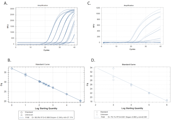
Figure 3: Standard curve and linear regression examples. A. Example of an acceptable standard curve derived from the amplification of three replicates each of six standard dilutions. A 10-fold standard dilution series with the highest concentration of the standard on the left, with decreasing concentrations moving to the right. The horizontal line crossing all the traces is the threshold for cycle at quantitation (Cq). Where each trace crosses this threshold is where the Cq is determined. B. Linear regression made from the standard replicates of Figure 3A. Replicates of the standard dilutions are plotted in circles and the unknowns (samples) are plotted with x’s. The efficiency is 98.9%, r² approaching 1.0, and slope of -3.349. C. Example of a poor standard curve derived from the amplification of three replicates each of six standard dilutions. D. A linear regression forming the standard curve for the standard replicates amplified in example 3C. Note the poor efficiency and r² values. Also note that only 4 of the 6 standards amplified. If after repeat runs, the standard curve does not improve, the problem may be with a poor primer/probe set that does not amplify target DNA as expected in which case, this assay should not be considered. Please click here to view a larger version of this figure.

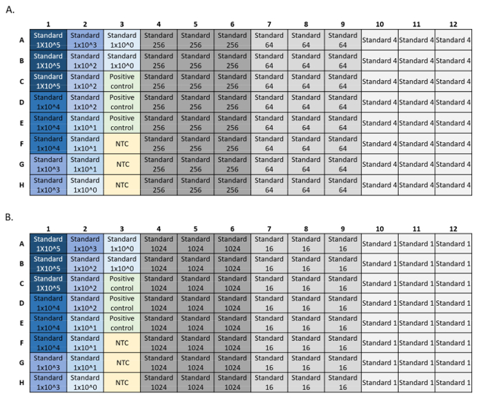
Figure 4: Examples of plate setups for LOD and LOQ standard qPCR runs. Standards used in the curve are in blue, standard concentration decreases from dark to light blue. DNA positive control in green and no template control (NTC) in yellow. Experimental standard concentrations in grey showing 24 replicates for each standard dilution. The dilution series was plated across two plates (A, B), each with a standard curve, positive control, and NTC. Please click here to view a larger version of this figure.

Figure 5: Plate setup and amplification traces from a qPCR run. A. Plate setup, standards shown in blue, darker color indicating the highest the concentration of the standard. DNA positive control in green, no template controls in yellow (NTC), sample targets in grey. B. Amplification traces from a qPCR run. Standards shown in blue, DNA positive control in green, no template controls in yellow, and unknowns in red. Please click here to view a larger version of this figure.

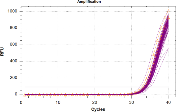
Figure 6: Amplification traces for the Internal Positive Control (IPC). IPC traces for all unknown samples in magenta and the IPC from the no template controls (NTCs) shown in orange with triangles. Please click here to view a larger version of this figure.

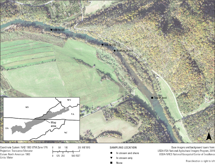
Figure 7: Map showing the eDNA collection sites of a mussel bed in the Clinch River along the Virginia/Tennessee border. Samples were collected at Wallens Bend at the bottom of the bed, 100 m downstream of the bed, and 500 m downstream of the bed. Sites were either collected in the middle of the stream (in stream) or roughly 1 – 2 meters from the shoreline (shore). Please click here to view a larger version of this figure.

Component	Name	Sequence 5’ – 3’		Fluorescent label
Forward Primer	A.lig.1-f	CCCTCATCACGTACCTCTTAATC
Reverse Primer	A.lig.1-r	GGAATGCCCATAATTCCAACTTTA
Probe	A.lig.1 probe	TTCTTGAACGTAAAGCCCTCGGGT		FAM

Table 1: The designed Actinonaias ligamentina qPCR assay (A.lig.1) including sequences for the forward and reverse primers and the probe.

Species	Amplified	In the Clinch River
1. Actinonaias ligamentina	Yes	Yes
2. Actinonaias pectorosa	No	Yes
3. Amblema plicata	No	Yes
4. Corbicula spp.	No	Yes
5. Cumberlandia monodonta	No	Yes
6. Cyclonaias tuberculata	No	Yes
7. Cyprogenia stegaria	No	Yes
8. Elliptio dilatata	No	Yes
9. Epioblasma brevidens	No	Yes
10. Epioblasma capsaeformis	No	Yes
11. Epioblasma florentina aureola	No	Yes
12. Epioblasma triquetra	No	Yes
13. Fusconaia cor	No	Yes
14. Fusconaia subrotunda	No	Yes
15. Lampsilis ovata	No	Yes
16. Lampsilis siliquoidea	No	No
17. Lasmigona costata	No	Yes
18. Lemiox rimosus	No	Yes
19. Lexingtonia dolabelloides	No	Yes
20. Medionidus conradicus	No	Yes
21. Plethobasus cyphyus	No	Yes
22. Pleurobema plenum	No	Yes
23. Ptychobranchus fasciolaris	No	Yes
24. Ptychobranchus subtentus	No	Yes
25. Quadrula pustulosa	No	Yes
26. Strophitus undulatus	No	Yes
27. Villosa iris	No	Yes

Table 2: A list of species used for the in vitro specificity testing of the A.lig.1 assay. The assay amplified genomic DNA of the target (Actinonaias ligamentina) and did not amplify any of the non-target species.

Component	Sequence 5’-3’
Actinonaias ligementina standard	CCCTCATCACGTACCTCTTAATCCTATTAGGTGTCGCATTTTTCACTCTTCTTGAACGTA
	AAGCCCTCGGGTACTTTCAAATCCGAAAAGGCCCAAATAAAGTTGGAATTATGGGCATTC
	CCCAACCATTAGCAGATGCTCTAAAGCTCTTCGTAAAAGAATGAGTAACACCAACCTCCT
	CAAACTACCTACCCTTCATCTTAACCCCAACCACTATGTTAATTTTAGCACTTAGACTTT
	GACAATTATTTCCATCCTTTATANTATCATCCCAAATANTTTTTGGTATGCTCCTATTCT
	TGTGTATCTCCTCCCTAGCTGTTTATACAACACTTATAACAGGCTGAGCCTCAAACTCCA
	AATATGCCCTTTTAGGAGCTATTCGAGCCATAGCCCAAACCATTTCTTATGAGGTTACAA
	TAAC
IPC template (Hem-T)	CTACATAAGTAACACCTTCTCATGTCCAAAGCTCTCTGAGTGTCCCTCGAATCTCAGACGCT
	GTATGACAGTCTCCTTTCGTGTGAACATTCGGCTGCTCTATGTTCTCAAGGACTGCAC

Table 3: Sequence (5’-3’) of the Actinonaias ligamentina standard and the IPC template (Hem-T) used for this assay. The sequence for the forward and reverse primers are in bold and italics, and that of the probe is underlined.

Component	Name	Sequence 5’ – 3’		Fluorescent label
Forward Primer	HemT-F	TCTGAGTGTCCCTCGAATCT
Reverse Primer	HemT-R	GCAGTCCTTGAGAACATAGAGC
Probe	HemT-P	TGACAGTCTCCTTTCGTGTGAACATTCG		Cy5

Table 4: The Internal Positive Control (IPC) assay including sequences for the forward and reverse primers and the probe.

Volume per sample (µL)	Component
10	Environmental Master Mix
1	20uM A. lig.1 F/R mix
1	2.5uM A. lig.1 probe
1	5uM IPC primer mix (HemT-F/ R)
0.75	2.5uM IPC probe (HemT-P)
1.5	1 X 103 concentration of the IPC template
2.75	H20
2	Sample
20	Total Volume

Table 5: The PCR mix used for the A.lig.1 assay multiplexed with the IPC assay.

Step		Temperature (°C )	Time
1	Initial Denature	95	10 min
2	Denature	95	15 sec
3	Annealing	60	1 min
4	Go to Step 2, repeat 39X

Table 6: Reaction conditions for the A.lig.1 assay.

Discussion

As with any study, defining the question to be addressed is the first step and the design of the eDNA assay depends upon the scope of the study²⁶. For instance, if the goal of the research or survey is to detect one or a few species, a targeted probe-based assay is best. If, however, the goal is to assess a larger suite or assemblage of species, high throughput sequencing metabarcoding assays are better suited. Once it is determined which approach to take, a pilot study including assay design, testing, and optimization is recommended²⁴. Assay design starts with a list of species as described in Figure 1. This list will be the basis for understanding how well an assay performs in terms of specificity and the geographic range it might be applied to^6,10. It is encouraged to design the assay for a specific geographic area, enabling the designer to better test an assay for cross-reactivity against other species in that area, and to be aware of the limitations this has on extending an assay to other areas where a target species may occur²⁴. Once the list is complete, sequences can be downloaded from public genetic databases. Since these databases are incomplete²⁷, one should sequence as many species on the list as possible in house to complete the local reference database of sequences that will be used in assay design. Prioritize co-occurring closely related species, as these are the most likely non-targets that will amplify. Focusing on all species within the same genus or family as the target species is a good place to start. Comparisons with closely related species will help identify sequence regions unique to the target species. This can help inform how the assay may perform in other systems or locations. Mitochondrial regions are the usual choice for assay development, because more sequence information from a wider variety of species is available at mitochondrial genes that have been used in barcode of life projects, and because mitochondrial DNA is present at much greater concentration in copies/cell than nuclear DNA^24,28,29. Multiple gene regions should be assessed for further assay development as sequence coverage varies among taxa in the genetic repository databases. After this local database of reference sequences is created, a combination of manual visualization of aligned sequence data and computer software programs is used to design the primer/probe assays. One should not rely strictly on software to determine which assays to test. It is important to verify visually on alignments where the primers and probes sit on the targets and non-targets to get a better understanding of how they might act in a PCR. Finally assay screening and optimization includes three levels (in silico, in vitro and in situ)^6,7,24,25. In silico design and testing are important for producing a short list of assays with a good chance of success, but empirical (in vitro) testing is crucial for selecting the assay with the best actual performance. In vitro optimization and testing of assays include measuring the reaction efficiency and defining the assay’s sensitivity and specificity. Limits of detection and quantification are two parameters often overlooked in assay development but important for data interpretation. By running multiple replicates of the standard curves for an assay, LOD and LOQ can easily be measured^1,5,30. Few studies discuss results with respect to the assay’s LOD or LOQ, but Sengupta et al. (2019) incorporate their assay’s LOD and LOQ into their data interpretation and graphics for a clearer understanding of their results³¹. Internal positive controls should be multiplexed into the designed assay as well. Without testing for PCR inhibition in the samples, false negatives may occur^24,32. We propose the use of a multiplexed IPC assay with the target assay as the easiest method for PCR inhibition testing²³. Finally, in situ testing of the assay from field and laboratory collected samples is necessary to ensure target amplification occurs in environmental samples²⁴.

Limitations exist for the use of species-specific, probe-based qPCR assays with eDNA samples. For instance, the design of multiple assays for testing may be limited by sequence availability, and compromise may be necessary on aspects of assay performance. These choices must be guided by the goals of the study and must be reported with the results²⁶. For example, if the goal is detection of a rare species and few positives are expected, an assay with imperfect specificity (i.e., amplification of non-target species) could be used if all detections will be verified by sequencing. If the goal is monitoring the geographic range of a species and eDNA concentration data is not needed, an assay with imperfect efficiency could be used and data reported only as percent detection. Furthermore, unless all potential conspecifics are tested in the laboratory, which is rarely possible, one cannot know with absolute certainty the true specificity of an assay. For instance, the assay was designed and tested against several freshwater mussel species in the Clinch River. To use this assay in a different river system, we would need to test it against a suite of species in the new location. Genetic variation within the species or population that is not tested during assay development might also affect specificity. Finally, even if an assay has been verified to have high technical performance; conditions change when working in the field. Non-assay related conditions such as water flow, pH, and animal behavior can change eDNA detectability as can use of different eDNA collection and extraction protocols. Using assays that are optimized and well described will help facilitate understanding of the influence such parameters have on eDNA detection.

The field of eDNA is maturing beyond the stage of exploratory analysis to increasing standardization of methods and techniques. These developments will improve our understanding of eDNA techniques, abilities, and limitations. The optimization process we outline above improves an assay’s sensitivity, specificity, and reproducibility. The ultimate goal of this refinement and standardization of eDNA methods is to improve researchers’ abilities to make inferences based on eDNA data as well as increase end-user and stake-holder confidence in results.

Materials

List of materials used in this article

Name	Company	Catalog Number	Comments
96 Place Reversible Racks with Covers	Globe Scientific	456355AST
Clean gloves (ie. latex, nitrile, etc.)	Kimberly-Clark	43431, 55090
CFX96 Touch Real-Time PCR Detection System	Bio-Rad	1855196
Fisherbrand Premium Microcentrifuge Tubes: 1.5mL	Fisher Scientific	5408129
Fisherbrand Premium Microcentrifuge Tubes: 2.0mL	Fisher Scientific	2681332
Hard-Shell 96-Well PCR Plates, low profile, thin wall, skirted, white/clear	Bio-Rad	#HSP9601
IPC forward and reverse primers	Integrated DNA Technologies, Inc.	none	custom product
IPC PrimeTime qPCR Probes	Integrated DNA Technologies, Inc.	none	custom product
IPC Ultramer DNA Oligo synthetic template	Integrated DNA Technologies, Inc.	none	custom product
Labnet MPS 1000 Compact Mini Plate Spinner Centrifuge for PCR Plates	Labnet	C1000
Microcentrifuge machine	Various	-	Any microcentrifuge machine that hold 1.5mL and 2.0mL tubes is typically okay.
Microseal 'B' PCR Plate Sealing Film, adhesive, optical	Bio-Rad	MSB1001
Nuclease-Free Water (not DEPC-Treated)	Invitrogen	AM9932
Pipette Tips GP LTS 1000 µL F 768A/8	Rainin	30389272
Pipette Tips GP LTS 20 µL F 960A/10	Rainin	30389274
Pipette Tips GP LTS 200 µL F 960A/10	Rainin	30389276
Pipettes	Rainin	Various	Depending on lab preference, manual or electronic pipettes can be used at various maximum volumes.
TaqMan Environmental Master Mix 2.0	Thermo Fisher Scientific	4396838
Target forward and reverse primers	Integrated DNA Technologies, Inc.	none	custom product
Target PrimeTime qPCR Probes	Integrated DNA Technologies, Inc.	none	custom product
Target synthetic gBlock gene fragment	Integrated DNA Technologies, Inc.	none	custom product. used for qPCR standard dilution series
TE Buffer	Invitrogen	AM9849
VORTEX-GENIE 2 VORTEX MIXER	Fisher Scientific	50728002

References

- Kubista, M., et al. The real-time polymerase chain reaction. Mol Aspects Med. 27 (2-3), 95-125 (2006).
- Higuchi, R. D., Walsh, P. S., Griffith, R. Simultaneous amplification and detection of specific DNA sequences. Biotechnology. 10, 5(1992).
- Mauvisseau, Q., et al. Influence of accuracy, repeatability and detection probability in the reliability of species-specific eDNA based approaches. Scientific Reports. 9 (1), 580(2019).
- Hernandez, C., et al. 60 specific eDNA qPCR assays to detect invasive, threatened, and exploited freshwater vertebrates and invertebrates in Eastern Canada. Environmental DNA. , (2020).
- Klymus, K. E., et al. Reporting the limits of detection and quantification for environmental DNA assays. Environmental DNA. , (2019).
- Thalinger, B., et al. A validation scale to determine the readiness of environmental DNA assays for routine species monitoring. bioRxiv. , (2020).
- Helbing, C. C., Hobbs, J. Environmental DNA Standardization Needs for Fish and Wildlife Population Assessments and Monitoring. CSA Group. , (2019).
- Sepulveda, A. J., Nelson, N. M., Jerde, C. L., Luikart, G. Are Environmental DNA Methods Ready for Aquatic Invasive Species Management. Trends in Ecology & Evolution. , (2020).
- Svec, D., Tichopad, A., Novosadova, V., Pfaffl, M. W., Kubista, M. How good is a PCR efficiency estimate: Recommendations for precise and robust qPCR efficiency assessments. Biomolecular Detection and Quantification. 3, 9-16 (2015).
- Wilcox, T. M., et al. Robust detection of rare species using environmental DNA: the importance of primer specificity. PLoS One. 8 (3), 59520(2013).
- Prediger, E. How to design primers and probes for PCR and qPCR. IDT. , Available from: http://www.idtdna.cco/pages/education/decoded/article/designing-pcr-primers-and-probes (2020).
- Thornton, B., Basu, C. Real-time PCR (qPCR) primer design using free online software. Biochemistry and Molecular Biology Education. 39, 145-154 (2011).
- Owczarzy, R., et al. IDT SciTools: a suite for analysis and design of nucleic acid oligomers. Nucleic Acids Research. 36, Web Server issue 163-169 (2008).
- Kibbe, W. A. OligoCalc: an online oligonucleotide properties calculator. Nucleic Acids Research. 35, Web Server issue 43-46 (2007).
- Taylor, S. C., et al. The Ultimate qPCR Experiment: Producing Publication Quality, Reproducible Data the First Time. Trends in Biotechnology. 37 (7), 761-774 (2019).
- Ye, J., et al. Primer-BLAST: A tool to design target-specific primers for polymerase chain reaction. BMC Bioinformatics. 13 (134), 11(2012).
- Altschul, S. F., Gish, W., Miller, W., Myers, E. W., Lipman, D. J. Basic Local Alignment Search Tool. Journal of Molecular Biology. 215, 403-410 (1990).
- Bustin, S. A., et al. The MIQE guidelines: minimum information for publication of quantitative real-time PCR experiments. Clinical Chemistry. 55 (4), 611-622 (2009).
- Bio-Rad. Bio-Rad Vol. 5279. , ed Bio-Rad (2020).
- Bio-Rad. Bio-Rad Vol. 6894. , Bio-Rad (2020).
- Eurogentec. Eurogentec. Vol. 0708-V2. , ed Eurogentec (2020).
- Bustin, S., Huggett, J. qPCR primer design revisited. Biomolecular Detection and Quantification. 14, 19-28 (2017).
- Hoorfar, J., et al. Practical considerations in design of internal amplification controls for diagnostic PCR assays. Journal of Clinical Microbiology. 42 (5), 1863-1868 (2004).
- Goldberg, C. S., et al. Critical considerations for the application of environmental DNA methods to detect aquatic species. Methods in Ecology and Evolution. 7 (11), 1299-1307 (2016).
- Guan, X., et al. Environmental DNA (eDNA) Assays for Invasive Populations of Black Carp in North America. Transactions of the American Fisheries Society. 148 (6), 1043-1055 (2019).
- Mosher, B. A., et al. Successful molecular detection studies require clear communication among diverse research partners. Frontiers in Ecology and the Environment. 18 (1), 43-51 (2019).
- Kwonga, S., Srivathsana, A., Meier, R. An update on DNA barcoding: low species coverage and numerous unidentified sequences. Cladistics. 28, 6(2012).
- Rees, H. C., et al. REVIEW: The detection of aquatic animal species using environmental DNA - a review of eDNA as a survey tool in ecology. Journal of Applied Ecology. 51 (5), 1450-1459 (2014).
- Evans, N. T., Lamberti, G. A. Freshwater fisheries assessment using environmental DNA: A primer on the method, its potential, and shortcomings as a conservation tool. Fisheries Research. 197, 60-66 (2018).
- Forootan, A., et al. Methods to determine limit of detection and limit of quantification in quantitative real-time PCR (qPCR). Biomolecular Detection and Quantification. 12, 1-6 (2017).
- Sengupta, M. E., et al. Environmental DNA for improved detection and environmental surveillance of schistosomiasis. Proceedings of the National Academy of Sciences of the United States of America. 116 (18), 8931-8940 (2019).
- Klymus, K. E., Richter, C. A., Chapman, D. C., Paukert, C. Quantification of eDNA shedding rates from invasive bighead carp Hypophthalmichthys nobilis and silver carp Hypophthalmichthys molitrix. Biological Conservation. 183, 77-84 (2015).
Reprints and Permissions