From Voxels to Knowledge: A Practical Guide to the Segmentation of Complex Electron Microscopy 3D-Data

Summary

The bottleneck for cellular 3D electron microscopy is feature extraction (segmentation) in highly complex 3D density maps. We have developed a set of criteria, which provides guidance regarding which segmentation approach (manual, semi-automated, or automated) is best suited for different data types, thus providing a starting point for effective segmentation.

Abstract

Modern 3D electron microscopy approaches have recently allowed unprecedented insight into the 3D ultrastructural organization of cells and tissues, enabling the visualization of large macromolecular machines, such as adhesion complexes, as well as higher-order structures, such as the cytoskeleton and cellular organelles in their respective cell and tissue context. Given the inherent complexity of cellular volumes, it is essential to first extract the features of interest in order to allow visualization, quantification, and therefore comprehension of their 3D organization. Each data set is defined by distinct characteristics, e.g., signal-to-noise ratio, crispness (sharpness) of the data, heterogeneity of its features, crowdedness of features, presence or absence of characteristic shapes that allow for easy identification, and the percentage of the entire volume that a specific region of interest occupies. All these characteristics need to be considered when deciding on which approach to take for segmentation.

The six different 3D ultrastructural data sets presented were obtained by three different imaging approaches: resin embedded stained electron tomography, focused ion beam- and serial block face- scanning electron microscopy (FIB-SEM, SBF-SEM) of mildly stained and heavily stained samples, respectively. For these data sets, four different segmentation approaches have been applied: (1) fully manual model building followed solely by visualization of the model, (2) manual tracing segmentation of the data followed by surface rendering, (3) semi-automated approaches followed by surface rendering, or (4) automated custom-designed segmentation algorithms followed by surface rendering and quantitative analysis. Depending on the combination of data set characteristics, it was found that typically one of these four categorical approaches outperforms the others, but depending on the exact sequence of criteria, more than one approach may be successful. Based on these data, we propose a triage scheme that categorizes both objective data set characteristics and subjective personal criteria for the analysis of the different data sets.

Introduction

Traditionally, the electron microscopy (EM) field has been divided into 1) the structural biology branch using high and super-high resolution TEM, typically combined with implicit or explicit data averaging to investigate the three-dimensional (3D) structure of macromolecular complexes with a defined composition and typically a relatively small size^1-4, and 2) the cellular imaging branch in which entire cellular sceneries are visualized^1,5,6. While the structural biology branch has undergone a spectacular development over the last four decades, the cell biology branch was mostly restricted to two dimensions, often on less-than-optimally preserved samples. Only with the advent of electron tomography in the last decade has cell biological ultrastructural imaging expanded into the third dimension^5,7, where typically averaging cannot be performed as the cellular sceneries, and thus the features of interest, are typically unique.

Although visualized cellular scenes are often stunning to the eye, efficient extraction of the features of interest and subsequent quantitative analysis of such highly complex cellular volumes lag behind, in part because the precise protein composition is usually unknown, therefore making it challenging to interpret these cellular 3D volumes. To this date, extensive biological expertise is often needed in order to interpret complex tomograms, or even to identify the important regions and essential components in the 3D volume. As a further complication, visualization of 3D volumes is remarkably non-trivial. 3D volumes can be thought of and thus visualized as stacks of 2D images. Slice-by-slice inspection of sequential 2D images reduces the complexity, but it also limits feature extraction and thus quantitative analysis to the two dimensions. However, for most 3D objects, the depiction of 3D volumes as merely a stack of consecutive planes leads to an incomplete and skewed perspective into a particular system’s 3D nature. Alternative modes of visual inspection require either volume rendering or surface rendering, which—given the often dense nature of a cellular volume—can easily lead to an obstructed view of nested objects or overwhelm a user altogether, thus making interactive manual segmentation difficult.

To remedy these barriers, a large variety of automated feature extraction (segmentation) approaches have been developed that are typically either density- or gradient-based^8-10. However, these methods tend to segment the entire volume regardless of which areas or features are of interest to the expert, although some recent methods can target a specific feature of interest such as actin filaments¹¹. In addition, the programs executing automated segmentation can sometimes result in the production of a large number of sub-volumes (e.g., when applying watershed immersion segmentation) that often need to be merged manually back into comprising the whole feature of interest or be subjected to further segmentation. This holds true particularly for complex and crowded data sets, thus most rendering computer algorithms are unable to extract only the features of interest with fidelity, and substantial curation efforts by an expert are often needed to produce a desired segmented volume.

Moreover, custom solutions to a highly specific problem are often published as a scientific meeting paper, with little to no emphasis on making them broad and comprehensive tools accessible to researchers who do not have intimate knowledge of the fields of mathematics, computer science and/or computer graphics. A customizable programming software environment, containing a range of image analysis libraries, can be a powerful tool set allowing users to efficiently write their own modules for accurate segmentation. However, this approach requires extensive training and a background in computer science in order to take advantage of its many features or capabilities for image analysis. One can work within such a versatile software environment for certain data sets where the features are more sparse, e.g., by utilizing powerful shape-based approaches which rely on the unique geometry of “templates” to separate objects of interest from their surroundings^12,13.

A fair variety of computer graphics visualization packages exist for interactive manual segmentation and model building. Some packages are commercially available, while others are of academic origin and distributed free of charge, such as: University of California San Francisco Chimera¹⁴, University of Colorado IMOD¹⁵, and University of Texas Austin VolumeRover¹⁶. However, the wide range and complexity of features and capabilities these programs possess steepens the learning curve for each. Certain visualization programs provide simple geometrical models, such as balls and sticks of various sizes, which can be placed into the density maps in order to create a simplified model of the complex 3D volume. These models then allow simple geometric and volumetric measurements and therefore go beyond just the “pretty picture”. Such manual tracing of objects works well for volumes where only a small number of objects need to be traced and extracted. However, the recent development of large volume 3D ultrastructural imaging using either focused ion beam scanning electron microscopy (FIB-SEM)^17-20 or serial block face scanning electron microscopy (SBF-SEM)²¹ presents the additional complication that the size of 3D data sets can range from gigabytes to tens and hundreds of gigabytes, and even the terabytes. Therefore, such large 3D volumes are virtually inaccessible to manual feature extraction, and hence efficient user-guided semi-automated feature extraction will be one of the bottlenecks for efficient analysis of 3D volumes in the foreseeable future.

Presented here are four different segmentation approaches that are routinely used on a large range of biological image types. These methods are then compared for their effectiveness for different types of data sets, allowing a compilation into a guide to help biologists decide what may be the best segmentation approach for effective feature extraction of their own data. As detailed user manuals are available for most of the programs described, the aim is not to make potential users familiar with any one of these particular packages. Instead, the goal is to demonstrate the respective strengths and limitations of these different segmentation strategies by applying them to six example data sets with diverse characteristics. Through this comparison, a set of criteria have been developed that are either based on the objective image characteristics of the 3D data sets, such as data contrast, crispness, crowdedness, and complexity, or stem from subjective considerations, such as the desired objective for segmentation, morphologies of the features to be segmented, population density of the features of interest, meaning the fraction of the volume occupied by the feature of interest, and how one proceeds optimally with finite resources such as time and availability of staff. These different example data sets illustrate how these objective and subjective criteria can be applied sequentially in a variety of combinations to yield a pairing of certain feature extraction approaches with certain types of data sets. The recommendations given will hopefully help novices faced with a large variety of segmentation options choose the most effective segmentation approach for their own 3D volume.

While the focus of this paper is feature extraction, attention to data collection and pre-processing data is crucial to efficient segmentation. Oftentimes staining of samples can be uneven, and hence, potential staining artifacts should be considered in the segmentation procedure. However, stain usually gives higher signal-to-noise, and therefore requires less filtering and other mathematical treatment of cellular volumes, which could potentially also result in artifacts. The respective raw image data sets need to be acquired at the correct contrast and camera pixel settings, aligned, and reconstructed into a 3D volume. For tomograms, aligned images are reconstructed typically using weighted back-projection, and then the data set is usually subjected to denoising algorithms such as non-linear anisotropic diffusion²², bilateral filtering²³, or recursive median filtering²⁴. FIB-SEM and SBF-SEM imaging data are aligned by cross-correlating consecutive slices in XY utilizing programs such as ImageJ²⁵. Contrast enhancement and filtering can be applied to boost the features of interest and thus to de-noise the image stack. Filtering can be performed either on the entire volume prior to subvolume selection or on the selected subvolumes, as filtering approaches can be computationally expensive. Down-sampling of the data (binning), which is sometimes used for noise reduction and/or file size reduction, is only recommended if the data has been significantly oversampled compared to the anticipated resolution.

After noise-reduction, the processed images can then be segmented by various methods, and the focus in this study is on the following four: (1) manual abstracted model generation through creating a ball-and-stick model, (2) manual tracing of features of interest, (3) automated threshold-based density, and (4) custom-tailored automated segmentation via a script for project specific segmentation. Boundary segmentation⁸ and immersive watershed segmentation¹⁰ are better alternatives to simple thresholding, but they belong in the same category and have not been included explicitly in this discussion.

 Manual tracing of densities requires outlining the features of interest, slice-by-slice, which allows the retention of the original density of respective sub-cellular areas. This approach allows maximal control of the segmentation process, but is a tedious and labor-intensive process.

Automated threshold-based (and related) density segmentation approaches are semi-automatic, where an algorithm chooses pixels based on a set of user-defined parameters. Several academic (free) visualization packages, such as UCSF Chimera, IMOD, Fiji²⁶, and VolumeRover are available, as well as commercial (requiring paid licenses) packages, and both types typically include one or more of these segmentation approaches. The software packages used in this work to illustrate these different methods include both commercial programs and academic open source programs for manually generating an abstract model, as well as manual and automated density segmentation. However, open source software can sometimes offer more advanced options through the possibility of customization.

A comparison of these techniques using different types of data sets led to the following presentation of rules and guidance on how to approach the segmentation of diverse biological data 3D volumes, which to our knowledge has not yet been published. Thus, this is the first systematic comparison of the different approaches and their usefulness on data sets with varying characteristics for users with different aims.

Protocol

1. Manual Abstracted Model Generation

Note: The details of the methodology described below are specific to Chimera, but other software packages may be used instead. Use this approach when the sole objective is to create a geometrical model (e.g., a ball and stick model) in order to make geometric measurements, rather than displaying the volume shape of the objects.

1. Import the data volume into a suitable program for manual abstracted model generation.
   1. Select File > Open Map to pull up the Open File dialog. Navigate to the file location of the desired map.
   2. Pull up the Volume Viewer (Tools > Volume Data > Volume Viewer) and select Features > Display Style to display data with different rendering styles.
   3. Adjust the threshold for the display by dragging the vertical bar on the histogram in the Volume Viewer window.
2. Navigate through the 3D volume (e.g., slice by slice) to select an area of interest for segmentation and crop out a smaller sub-volume if necessary.
   1. In the Volume Viewer dialog, click Axis, then select X, Y, or Z.
   2. In the Volume Viewer dialog, select Features > Planes. Click One to set Depth to display the plane corresponding to the number in the left box, and click All to display all planes.
   3. In the Volume Viewer dialog, select Features > Subregion selection.
      1. Click and drag to create a rectangular box around the region of interest.
3. Place markers along the feature of interest and connect them with linkers where appropriate (often done automatically by the program) until the model is complete.
   1. From the Volume Viewer menu bar, select Tools > Volume Tracer dialog to open the Volume Tracer dialog. In the Volume Tracer dialog, select File > New Marker Set.
   2. In the Volume Tracer dialog, check Mouse > Place markers on high quality, Place markers on data planes, Move and resize markers, Link new marker to selected marker, and Link consecutively selected markers.
   3. Click on the Marker Color swatch, and select a color. Repeat this step for Link color.
   4. Enter radii for the marker and link model-building elements.
   5. In the Volume Tracer Window, select Place markers using [right] mouse button, and insert radii for markers and links.
   6. Right click on the volume data to begin laying down markers. Markers will be connected automatically.
   7. In the Volume Tracer dialog, select File > Save current marker set, then File > Close marker set.
4. Open a new marker set (Step 1.3.1) to begin building a model into a second desired feature of interest. Utilize contrasting colors between marker sets to emphasize differences in features.

2. Manual Tracing of Features of Interest

Note: The details of the methodology described below are specific to Amira, but other software packages may be used instead. Use this approach when the population density is relatively small and when accuracy of feature extraction is paramount, as manual tracing is a time-consuming approach.

1. Import volume data into a program with manual tracing options. Software with this capability generally offer at least a basic paintbrush tool.
   1. For large volumes or tomograms (e.g., 16-bit 2,048 x 2,048 or larger .rec or .mrc tomograms generated in IMOD): Select Open Data > Right click on filename.rec > Format… >Select Raw as LargeDiskData > Ok > Load. Select appropriate Raw Data Parameters from header information > Ok. Toggle and Save As a new filename.am file for use in the following steps.
   2. For smaller 3D image stack files (e.g., 3D .tif or .mrc or .rec): Open Data > Select filename.tif or filename.mrc. Toggle and Right Click > Save As filename.am. If an error is generated or the program is unresponsive, the file may be too large and can be opened by following Step 2.1.1.
2. Navigate through the slices to select a 3D sub-volume for segmentation, and then crop to this area of interest.
   1. In 3D Viewer window, select Orthoslice to open image file. Use slider at bottom to navigate through slices.
   2. To crop larger data opened as LargeDiskData, toggle file name in Pool window > Right click > LatticeAccess. Enter desired box size > Apply. Save new file.
3. Create segmentation file.
   1. Toggle the file in the Pool window > Right Click > Labeling > LabelField. A new file will be created and automatically loaded in the Segmentation Editor tab.
4. Trace the border of the first feature of interest, then fill the trace by hand or by using a command specific to the software used. Follow the feature of interest through all slices and repeat the manual tracing segmentation. Use the following commands when using Amira:
   1. To use the Paintbrush tool, alter brush size as desired, then use the mouse pointer to trace the border of the feature of interest.
   2. Fill the traced area with shortcut “f”. Add the selection by clicking the button with the plus symbol, or the shortcut “a”. If necessary, press “u” to undo, and “s” to subtract or erase.
5. Generate a surface rendering for visualization and basic qualitative or quantitative analysis per software user guide instruction.
   1. In the Object Pool tab, toggle the filename-labels.am in the Pool window > Right click > SurfaceGen.
   2. Select desired Surface properties > Apply. A new file filename.surf will be created in the Pool.
   3. To visualize the segmented volume, toggle filename.surf in Pool window > Right click > SurfaceView.
   4. Use the tools in the 3DViewer window to move, rotate, and zoom in the 3D volume.
6. Extract the exact densities and determine measurements such as volume or surface area. Export to other programs for more advanced display, analysis and simulation.
   1. On 3DViewer window, click Measure tool > Select appropriate option (2D length and 2D angle for measurements on a single 2D plane, 3D length and 3D Angle for measurements on a 3D volume).
   2. Click on mesh surface to measure desired length, distance, and angles. The values will be listed in the Properties window.

3. Automated Density-based Segmentation

Note: The details of the methodology described below are specific to Amira, but other software packages may be used instead.

1. Use this approach on data sets with any variety of contrast, crispness, or crowdedness to withdraw the densities of interest.
2. Import volume data into a program equipped with thresholding, magic wand, or other density-based tools for automatic segmentation. Follow steps outlined in 2.1-2.1.2 in the directions for manual tracing.
3. Navigate through slices and select area for segmentation. If necessary, crop out a smaller 3D sub-volume for segmentation. Follow steps outlined in 2.2-2.2.2 in the directions for manual tracing.
4. Select the density of a feature of interest, usually by clicking or placing a mark or anchor point on the feature. If allowed in the software, enter a number range encompassing the feature’s pixel intensity and adjust this tolerance as desired. Densities belonging to the feature will be picked up in accordance to the intensity of the anchor’s pixel or tolerance value. Use the following commands when using Amira.
   1. Use the Magic Wand Tool for features with distinguishable margins.
      1. Click on the area of interest, then adjust sliders in Display and Masking to capture correct range of values so that the feature is fully highlighted. Add selection with shortcut “a”.
   2. Use the Threshold Tool for features without clearly distinguishable margins.
   3. Select the Threshold icon. Adjust slider to adjust density within desirable range so that only the features of interest are masked. Click Select button, then add selection with shortcut “a”.
   4. To segment entire volume, select All slices before adding selection.
   5. To remove noise, select Segmentation > Remove Islands and/or Segmentation > Smooth labels.
5. Generate a surface for visualization and qualitative analysis as described in the manual tracing section 2.6-2.6.2. If desired, export to other programs for adequate 3D display, quantitative analysis and simulations.

4. Custom-tailored Automated Segmentation

Note: Use this approach to create customized scripts for automatic segmentation, which requires background experience in computer science, but allows the ability to create a precise density model from a large volume.

1. Tools (Specific Example of Shape-Supervised Segmentation in MATLAB²⁷)
   1. Image pre-processing: Perform de-noising, background removal and image enhancement by using the following pipeline:
      1. Load the image using the imread command.
         1. In the command line, enter: >> im = imread($image_path), where $image_path is the location of the image to be analyzed.
      2. From the Image Processing toolbox, call Wiener Filter using an estimated or known Noise-power-to-signal ratio (NSR).
      3. On the previously processed image, call the image opening function imopen to estimate the background layer, then allocate the outcome as a different mask.
         1. In the command line, enter: >> background = imopen(im,strel($shape_string,$size)), in this method, $shape_string is equal to ‘disk’ the variable $size is given by the analyzer. i.e. >> background = imopen(im,strel(‘disk’,15)).
      4. Subtract the filtered image with the background.
         1. In the command line, enter: >> im2 = im - background
      5. Depending on the quality of the results, perform image normalization with or without adaptive Otsu’s method²⁸, which can be called using the function imadjust from the Image Processing Toolbox.
         1. In the command line, enter: >> im3 = imadjust(im2)
      6. Prepare the features of interest for segmentation, limiting the regions of interest by cropping the normalized image.
         1. Using the imtool command, explore the region of interest that is to be cropped and provide the coordinates to the command: >> im3_crop = imcrop(im3, [x1 y1 x2 y2]), where the vector [x1 y1 x2 y2] corresponds to the square region to be cropped.
   2. Shape recognition/Supervised shape classification: Train the algorithm by providing specific examples for each different category of objects (linear traces in a 2D image across the features of interest).
      1. Check that VLFEAT²⁹ API is successfully installed and visit VLFEAT’s website for more in-depth documentation.
      2. In the command line, enter: >> [TREE,ASGN] = VL_HIKMEANS(im3_crop,$K,$NLEAVES) where $K is the number of cluster to be used or the number of classes the observer wants to arrange the data into, and $NLEAVES is the desired number of leaf clusters i.e. >> [TREE,ASGN] = VL_HIKMEANS(im3_crop,4,100)
      3. Use manually segmented features as the input for VLFeat.
         NOTE: This open source C-based library will perform pixel patching, patch clustering, and cluster center positioning depending on the type of method chosen to work best for the datasets. The available options range from k-mean clustering to texton-based approaches³⁰, and the output is a numerical array that describes the features desired based on the given exemplars.
2. Segmentation: Use this fully automated, although computationally expensive, approach to segment multiple classes of objects simultaneously, which will be written out as separate maps for further visualization and analysis.
   1. Load the previously generated numeral array (model).
   2. Call the support vector machine (SVM) function in VLFeat, using the model and the image to be segmented as an input.
      1. In the command line, enter: >> [w, b] = vl_svmtrain(x, y, 0.1), where x is the original cropped image im2_crop and y is the objective image, the image that has been manually segmented. Use >> ISEG = VL_IMSEG(I,LABELS) to color the results according to the labels generated by the clustering.
         NOTE: Based on the characteristics of the model, VLFeat will classify the image on the number of classes (features of interest) assigned from the beginning. Depending on the grade of accuracy desired, it is possible to combine this method with other approaches or estimate cluster parameters such as hull and cluster centers. The output of the SVM algorithm is a probabilistic model and multiple binary masks of the desired classes in the new datasets.
   3. Save results by entering the command: >> imwrite(im, $format, $filename) where $format is 'tiff' and $filename is the path for the output file.
   4. For visualizing images, enter the command: >> imshow(im).

Results

Figure 1 shows a typical workflow for 3D electron microscopy cellular imaging, including electron tomography, FIB-SEM, and SBF-SEM. The workflow includes raw data collection, data alignment and reconstruction into a 3D volume, noise reduction through filtering, and when necessary, cropping to the region of interest in order to maximize the effectiveness of the chosen segmentation software. Such preprocessed data is then ready for feature extraction/segmentation.

Figure 2 illustrates the workflow laid out in Figure 1 with four different data sets (which will be introduced further below), two of which are resin-embedded samples recorded by electron tomography (Figures 2A, 2B), with the other two stemming from FIB-SEM and SBF-SEM, respectively (Figures 2C, 2D). Images in Figure 2 column 1 are projection views (Figures 2A1, 2B1) and block surface images (Figures 2C1, 2D1), respectively, which upon alignment and reconstruction are assembled into a 3D volume. Column 2 shows slices through such 3D volumes, which upon filtering (column 3) show a significant reduction in noise and thus often appear more crisp. After selecting and cropping the large 3D volume to the region of interest (column 4), 3D renderings of segmented features of interest (column 5) can be obtained and further inspected, color coded and quantitatively analyzed.

A total of six 3D data sets, each containing a stack of images obtained through either electron tomography (3 data sets), FIB-SEM (2 data sets), or SBF-SEM (1 data set) are used to compare how each of the four segmentation methods perform (Figure 3). The data sets stem from a variety of different research projects in the laboratory and thus provide a reasonably diverse set of typical experimental data sets. All data sets were examined by four independent researchers, each of whom are most familiar with one particular approach, and they were charged with providing the best possible result for each of the six data sets.

The data sets are from samples as follows: 1. Figures 3A1-3A5: high pressure-frozen, freeze-substituted and resin-embedded chick inner ear hair cell stereocilia³¹, 2. Figures 3B1-3B5: high pressure-frozen, freeze-substituted and resin-embedded plant cell wall (unpublished), 3. Figures 3C1-3C5: high pressure-frozen, freeze-substituted and resin-embedded inner ear hair cell kinocilium (unpublished), 4. Figures 3D1-3D5: high pressure-frozen, freeze-substituted and resin-embedded blocks of mitochondria located in human mammary gland epithelial cells HMT-3522 S1 acini, which have been cultured in laminin rich extracellular matrix^32,33, 5. Figures 3E1-3E5: unstained benchtop-processed, resin-embedded blocks of a sulfate reducer bacterial biofilms (manuscript in preparation), and 6. Figures 3F1-3F5: membrane boundary of neighboring cells of the HMT-3522 S1 acini.

As can be seen from Figure 3, different segmentation approaches can lead to mostly similar results for some data set types, but completely different results for other data types. For example, the hair cell stereocilia data set (Figure 3A) yields reasonable segmentation volumes with all four approaches, with the manual abstracted model generated by an expert user being the clearest to interpret and measure. In this case, such a model allows for quick measurements of filament-filament distances, counting of the number of links found between the elongated filaments, as well as determination of missing parts of the density map corresponding to locations where the specimen was damaged during sample preparation³⁴. Such information is much more difficult to acquire by using the other three segmentation approaches, although the custom-tailored automated segmentation provides better results than purely density-based thresholding.

For the plant cell wall (Figure 3B), manual model generation appeared to be the most efficient in conveying a sense of order in the cell wall, which none of the other approaches achieve. However, the abstracted model does not capture the crowdedness of the objects in the data set. Manually tracing features of interest seems to give a better result than the density-based or shape-supervised approaches. On the other hand, manual tracing is very labor-intensive and identifying borders of the features is somewhat subjective. Therefore, automated approaches may be preferred for segmenting large volumes with a potential trade-off between precision and resources spent on manual segmentation.

For the kinocilium data set (Figure 3C), manual abstracted model generation yields the cleanest result and reveals an unexpected architecture of three microtubules at the center of the kinocilium, a detail that is readily visible in the cropped data, but lost in all other approaches, presumably due to stain heterogeneity. However, other potentially crucial features of the density map are missed in the manual generation of an abstract model. This is due to the fact that the subjective nature of manual model formation leads to an idealization and abstraction of the actual density observed, and therefore to a subjective interpretation during the model formation. Hence, this example nicely demonstrates how manual abstracted model generation allows one to concentrate on a specific aspect of the 3D volume. However, the selective perception and simplification fails to give a full account of all the protein complexes present in the data set. Therefore, if the objective is to show the complexity of the data, then one is better served with any of the other three approaches.

In the case of the 3D matrix-cultured mammary gland acini (Figure 3D), the high contrast mitochondria are segmented by all four approaches with ease, with the manual tracing of features not too surprisingly yielding the best results with the lowest amount of contamination (Figure 3D3). However, manual tracing is very labor-intensive and is therefore of limited use for large volumes. Both density threshold-based and shape-supervised automated segmentation extract the mitochondria quite well, and would result in a near-perfect segmentation, if further tricks for cleanup are employed (e.g., eliminating all objects below a particular threshold of voxel density) as available in different packages. In this case, manual abstracted model building did not yield promising results, in part because mitochondria cannot easily be approximated with ball and stick models.

With respect to the bacterial soil community/biofilm (Figure 3E), three of the four approaches yield reasonable results, with the manual model generation not performing well due to the challenge of representing biological objects, such as bacteria, by geometrical shapes. Extracellular appendages originating from the bacteria can be detected in the automated segmentation approaches but not as well in the manual feature tracing. Shape-supervised custom-tailored automated segmentation can further separate the extracellular features from the bacteria despite their similar densities (data not shown), allowing easy quantification even of extremely large data sets. Because this is originally a very large data set, the custom-tailored automated segmentation clearly outcompeted all other approaches, but may have benefited from the low complexity and the relatively sparse distribution of the objects of interest (low crowdedness).

When examining the interface between two eukaryotic cells in a tissue-like context (Figure 3F), only the manual tracing of features of interest produced good results. Automated density-based segmentation approaches fail to detect the membrane boundary between adjacent cells altogether, and even the custom-tailored approaches fails, in part because the shape of a cell is not easily approximated or equated with shapes, despite its clear success for the bacteria in the biofilm (Figure 3E5).

The observation from Figure 3 that the segmentation approaches do well on some data sets but not on others led to the question of what characterizes each of these data sets, and whether it was possible to categorize the types of data characteristics or personal aims that appeared to match well with their respective approach. Systematic study of this topic has not been previously conducted, and thus as a first step an establishment of an empirical list of image characteristics and personal aims may guide a novice in their attempt to find the best approach for feature extraction of their respective data set.

Eight criteria were identified as significant are shown in Figure 4, and they can be divided into two main categories: (1) the features that are inherent in the data set, and (2) the researcher’s personal objectives and other considerations that are somewhat more subjective, albeit equally important. The examples shown are predominantly drawn from the six data sets in Figure 3, with three additional data sets being introduced: one (Figure 4A1) is a cryo-tomogram of a cryo-section of Arabidopsis thaliana plant cell wall, the second (Figures 4A2, 4B1, 4D1) is a FIB/SEM data set of the inner ear stria vascularis, which is a highly complex and convoluted tissue that could fit in the category depicted in Figures 3F1-3F5 but is even more substantially complex, and the third (Figures 4B2, 4D2) is a resin-section tomogram of inner ear hair cell stereocilia in cross-sectional view, similar to the sample content shown in longitudinal view in Figuress 2A1-2A5 and 3A1-3A5.

For the category of the objective criteria like image characteristics, four traits inherent in the data sets are proposed to be of importance:

1. The data contrast can be (1) low (Figure 4A1) as is typical for cryo-EM tomograms, (2) intermediate (Figure 4A2) such as in cellular sceneries with no clear organelle or other prominent feature standing, or (3) high (Figure 4A3), as is the case for the kinociliary tomogram or the stereocilia in cross section, due to the alignment of clearly separated filamentous elements within the z-direction.
2. The data can be fuzzy (Figure 4B1), with no visibly clear boundaries between two closely positioned objects, such as cells in a tissue, or crisp (Figure 4B2), with sharply defined boundaries. This is partly a function of the data set resolution, which is inherently higher by a factor of about 2-4 for electron tomograms compared to FIB-SEM. Naturally, sharper boundaries are desirable for both manual as well as automated segmentation approaches, but essential for the latter approach.
3. The density maps can be either crowded (Figure 4C1) as reflected by the tightly spaced plant cell wall components, or sparsely populated (Figure 4C2), as are the bacteria in a colony, which exemplifies the separation that renders automated image segmentation substantially easier.
4. Density maps can be highly complex with vastly different features often with irregular shapes, such as the stria vascularis tissue around a blood vessel (Figure 4D1) or well-defined organelle-like objects with a similar organization, such as the stereocilia in cross section (Figure 4D2).

Also note the vastly different scales in all the different examples, making the comparison somewhat difficult.

Apart from the more objective criteria such as image characteristics, four highly subjective criteria that will guide the selection of the appropriate path are also proposed:

1. Desired Objective: The objective may be to visualize the hair bundle stereocilium in its complexity and to determine and examine the shape of the object (Figure 4E1), or to create a simplified and abstracted ball and stick model that is built into the density map and allows a fast counting and measuring of the geometrical objects (filament length, distance and number of connections) (Figure 4E2).
2. The feature morphology can be highly irregular and complex like cells, such as cell-cell interaction zones (Figure 4F1), somewhat similarly shaped with some variation, such as mitochondria (Figure 4F2), or mostly identically shaped, such as actin filaments and cross links in a hair bundle in longitudinal orientation (Figure 4F3).
3. The proportion of the feature of interest (population density) is important, as one may want to segment all features in a 3D data set, as is the case for plant cell walls (Figure 4G1), or only a tiny fraction of the cellular volume as is the case of mitochondria in a heterogeneous cellular scene (Figure 4G2). Depending on the size of the data set and the percentage of volume that requires segmentation, it may be most efficient to use manual approaches. In other cases, such as when one is interested in a variety of features, there is simply no alternative to using semi-automated segmentation approaches.
4. Another key subjective criterion is the amount of resources one is willing to invest into the segmentation process and what level of fidelity is required to answer a biological question. One may want and need to quantify a feature’s volumetric parameters (such as size, volume, surface area, length, distance from other features, etc.), in which case more care may be needed to obtain accurate quantitative information (Figure 4H1), or the purpose may be to merely snap a picture of its 3D shape (Figure 4H2). In an ideal world where resources are unlimited, one clearly would not want to make any compromises but rather opt for the most accurate path of user-assisted manual feature extraction. While this can work for many data sets, in the near future 3D volumes will be in the order of 10k by 10k by 10k or higher, and manual segmentation will no longer be able to play a prominent role in segmenting such an enormous space. Depending on the complexity of the data and other data characteristics, semi-automated segmentation may become a necessity.

In Figure 5, strengths and limitations are briefly listed for the four segmentation approaches. The personal aims and image characteristics identified in Figure 4 that can pair with each approach are outlined as well. In Figure 6, the personal aims and image characteristics of the six datasets exemplify how to triage data and decide on the best approach. Both Figures 5 and 6 are expanded upon in the discussion.

Figure 1. Workflow for biological imaging reconstruction and analysis. This chart gives an overview of the various steps taken to collect and process images collected by tomography, focused ion beam SEM, and serial block face SEM. Raw data collection results in 2D tilt series or serial sections. These 2D image sets must be aligned and reconstructed into 3D, then filtered in order to reduce noise and enhance the contrast of features of interest. Finally, the data can be segmented and analyzed, ultimately resulting in a 3D model. Please click here to view a larger version of this figure.

Figure 2. Examples of workflow for different data types from tomography and FIB-SEM. Each step of the workflow after data collection is shown through four data sets (rows A-D): resin embedded stained tomography of longitudinally sectioned stereocilia, resin embedded stained tomography of plant cell wall cellulose, FIB-SEM of breast epithelial cell mitochondria, and SBF-SEM of E. coli bacteria. A 2D slice through the raw data is shown in column 1, and an image from the data after alignment and 3D reconstruction comprises column 2. The filtering techniques applied in column 3 are the following: median filter (A3), non-anisotropic diffusion filter (B3), Gaussian blur (C3), and MATLAB’s imadjust filter (D3). An example of the best segmentation for each data set from the cropped area of interest (column 4) is displayed as a 3D rendering in column 5. Scale bars: A1-A3 = 200 nm, A4 = 150 nm, A5 = 50 nm, B1-B3 = 200 nm, B4-B5 = 100 nm, C1-C3 = 1 mm, C4-C5 = 500 nm, D1-D3= 2 mm, D4-D5 = 200 nm. Please click here to view a larger version of this figure.

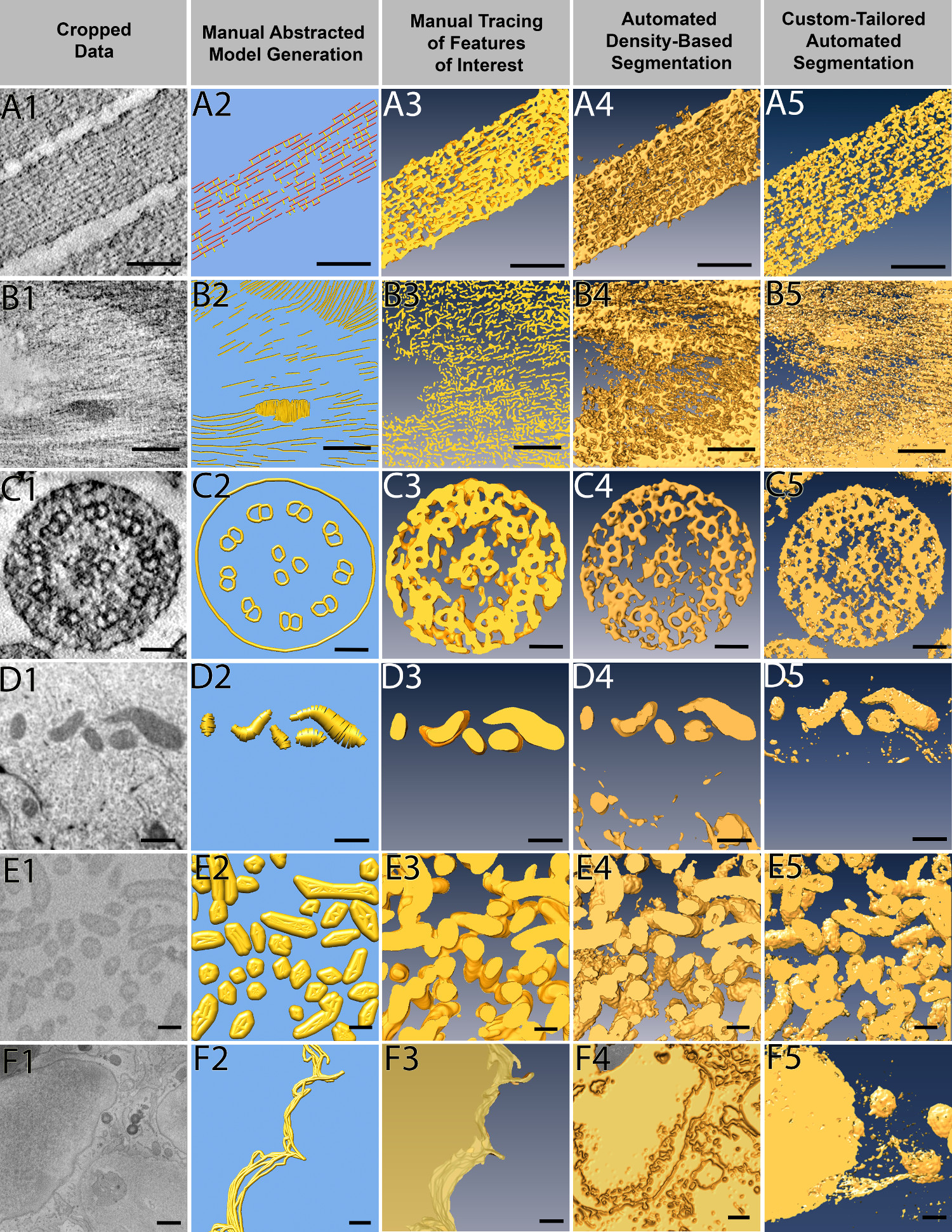
Figure 3. Application of four segmentation approaches to example data sets. Six example data sets were segmented by all four approaches: manual abstracted model generation, manual tracing, automated density-based segmentation, and custom-tailored automated segmentation. Manual abstracted model generation was effective for the resin embedded stained tomography of stereocilia (A), as the purpose was to create a model for quantitative purposes rather than to extract densities. For the resin embedded stained tomography of plant cell wall (B), automated density-based segmentation was the most effective method to quickly extract the cellulose through many slices, where as the manual methods took much more effort on only a few slices of data. Manual abstracted model generation generated the microtubule triplet in the stained tomography of kinocilium (C) while other segmentation methods did not, yet the two automated approaches extracted the densities more quickly and were therefore preferred. Due to the shape of mitochondria from FIB-SEM of breast epithelial cells (D), manual tracing provided the cleanest result, and the low population density combined with use of interpolation methods allowed for quick segmentation. Given the large volume that needed to be segmented, custom-tailored automated segmentation proved to be most efficient to segment the SBF-SEM bacteria data (E), but both automatic approaches were comparable. Although time consuming, the only method to extract the FIB-SEM of breast epithelial cell membrane (F) was manual tracing. Scale Bars: A1-A5 = 100 nm, B1-B5 = 100 nm, C1-C5 = 50 nm, D1-D5 = 500 nm, E1-E5 = 200 nm, F1-F5, bars = 500 nm. Please click here to view a larger version of this figure.

Figure 4. Objective image characteristics and subjective personal aims for triaging of data sets. Using examples of data set characteristics, criteria are proposed to inform a decision as to which segmentation approach to use. With respect to objective characteristics, data can inherently have contrast that is low, medium, or high (A1-A3), be fuzzy or crisp (B1-B2), spaced out or crowded (C1-C2), and have complex or simply organized features (D1-D2). Subjective personal aims include the desired objective targeting a simplified model or extracting the exact densities (E1-E2), identifying a convoluted sheet, convoluted volume, or linear morphology as the feature of interest (F1-F3), choosing a high or low population density of the feature of interest (G1-G2), and deciding upon the trade-off between high-fidelity and high-resource-allocation for a diminishing return on investments such as time (H1-H2). Scale Bars: A1= 50 nm, A2 = 1500 nm, A3 = 100 nm, B1 = 1500 nm, B2 = 200 nm, C1 = 100 nm, C2 = 200 nm, D1 = 10 mm, D2 = 200 nm, E1 = 100 nm, E2 = 50 nm, F1-F2 = 500 nm, F3 = 50 nm, G1 = 100 nm, G2 = 1 mm, H1-H2 = 100 nm. Please click here to view a larger version of this figure.

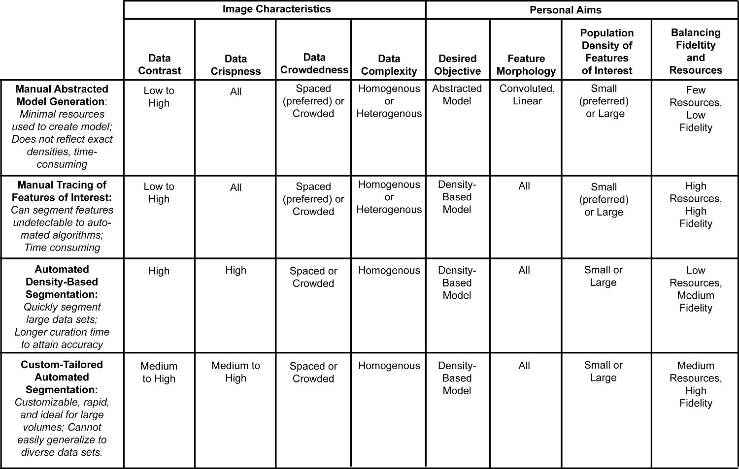
Figure 5. Comparison table of data characteristics and subjective aims appropriate for different segmentation approaches. This table summarizes the strengths and limitations of each segmentation approach. The criteria from Figure 4 can help identify which datasets are suitable for which segmentation method. These objective image characteristics and subjective personal aims were chosen for optimal use of each approach, but different combinations may hinder or aid the efficiency of the segmentation. Please click here to view a larger version of this figure.

Figure 6. Decision flowchart for efficient triage of segmentation approaches for data sets with varying characteristics. Based upon the characteristics highlighted in Figure 4, this diagram illustrates which four criteria contributed the most to the final decision on the best segmentation approach for each data set from Figure 3. Each data set is color coded to quickly follow the bold lines representing the primary decision-making process, as well as the dotted lines that reflect an alternate path that may or may not lead to the same approach. The kinocilium, bacteria, and plant cell wall data sets were best segmented with the two automated approaches. In contrast, the cell membrane and mitochondria paths always lead to manual tracing due to their difficult characteristics. Please click here to view a larger version of this figure.

Discussion

Effective strategies for the extraction of relevant features from 3D EM volumes are urgently needed in order to keep up with the data tsunami that has recently hit biological imaging. While data can be generated in hours or days, it takes many months to analyze the 3D volumes in depth. Therefore, it is clear that the image analysis has become the bottleneck for scientific discoveries; without adequate solutions for these problems, imaging scientists become the victims of their own success. This is in part due to the high complexity of the data and also the macromolecular crowding typically found in biological cells, where proteins and protein complexes border one another and essentially appear as a continuous gradient of grayscale densities. The problem is complicated by sample preparation and imaging imperfections, and in some cases image reconstruction artifacts, leading to less than perfect volumetric data that can pose challenges for fully automated approaches. Most significant, however, is the fact that the experts in sample preparation, imaging, and the biological interpretation are seldom well versed in computational science, and hence require guidance on how to effectively approach feature extraction and analysis. Therefore, through the use of various examples, the protocol explains how to prepare data for segmentation, as well as the steps for manual abstracted model generation, automated density-based segmentation, manual tracing of features of interest, and custom-tailored automated segmentation. The manual and automatic approaches outlined in the procedure can be found in a large variety of segmentation software, some of which are mentioned here, but others perform similar functions and are equally well suited.

The results demonstrate that the effectiveness of each of the 3D segmentation approaches varies for each different type of data sets. Even though the different approaches produced qualitatively similar 3D renderings as the end product, the amount of time and effort spent on each during the segmentation process varied significantly. The recommendations for appropriate image characteristics and personal aims per segmentation approach are summarized in Figure 5, which is further explained in the following four subsections. These criteria were applied to the six datasets, as shown in the decision flow chart of Figure 6. Although Figures 5 and 6 are merely meant to provide a rationale for each data set and how each of the criteria were weighted in the decision making process, they do not provide a foolproof guidance, but rather a starting point. There are simply too many criteria that influence the decision-making process: some are objective criteria, such as data set characteristics, whereas others are more subjective criteria, such as the desired objective. It is safe to say that data sets that display a high level of contrast with sharp crisp boundaries, have features that are well separated and relatively homogeneous (not too diverse), and are processed with the objective of displaying a density model for a large number of objects, automated approaches will be superior, if not for the fact that manual approaches would simply be resource (time)-prohibitive. On the other hand, if contrast is low, the data is fuzzy and thus requires an expert’s knowledge, the objects are crowded, and the features show a high diversity and are thus heterogeneous, one may not have any other choice than manual feature extraction/segmentation.

Manual Abstracted Model Generation

Manual abstracted model tracing is particularly effective in segmenting linear elements, providing seeds points (balls) that can be automatically connected (sticks). Such balls and sticks-models can be very powerful to measure length and orientation of such model and provide an adequately abstracted model for both qualitative inspection and quantitative analysis. Manual abstracted model generation is commonly used when minimizing resources spent on the analysis is more important than absolute fidelity to the shapes of the original data. It is most successful with linear and homogenous features of interest (e.g., filaments, tubes). Data contrast, crispness, and crowdedness do not play a major role in determining this method’s success, as long as the human eye can recognize the object of interest. Sometimes such models can also be utilized as a skeleton to segment the 3D map in a zone around the skeleton. Although the model is abstract rather than a reflection of exact densities, it represents a skeletonized version of the 3D density and thus allows for clutter-free visualization and qualitative analysis. Quantitative measurements such as length can also be determined from the approximate model. For an example of software with manual abstracted model generation, please visit Chimera’s detailed user guide online at http://www.cgl.ucsf.edu/chimera/current/docs/UsersGuide/index.html.

Manual Tracing of Features of Interest

Manual paintbrush tracing works well with almost all data characteristics, but it is also the most time consuming method. At times, it is the only technique for extracting a feature of interest from a complex image set containing a large variety of features, such as the thin and convoluted cell membrane. One useful tool available in some programs allows for interpolation between intermittently segmented slices when the feature of interest changes smoothly. Manual tracing can be applied most efficiently if the data is crisp and has medium to high contrast, but it can also be utilized for more challenging data sets, as long as the user is familiar with the object of interest. The data complexity can range from discrete objects to complex and crowded data sets, where objects are closely packed. In the latter case, manual segmentation may be the only choice, as automatic approaches often struggle to segment the desired volume and extract too much or too little. Difficult feature morphologies, such as convoluted sheets or volumes, can also be extracted by this method. However, the user should keep in mind that a dataset with several difficult characteristics can only be segmented if the population density of the features of interest is low, as segmentation of high population densities of the features of interest becomes time-prohibitive. For an example of software with manual tracing, please visit Amira’s detailed user guide online at http://www.vsg3d.com/sites/default/files/Amira_Users_Guide.pdf.

Automated Density-based Segmentation

In contrast to the manual techniques, the automated approaches are generally less time-consuming, which is an important factor to consider when segmenting a large stack of images. However, simple thresholding may not be as accurate, and much more time may be spent on refinement and curation of the automatically segmented volume. Automated density-based segmentation works best on data sets that display a large number of similar features of interest that all require segmentation. If the data is more complex, these automated techniques can still serve as an initial step, but will likely require some manual intervention down the line in order to specify a subvolume containing the feature of interest. This strategy typically works well on linear morphologies or convoluted volumes, but it is rarely successful with thin convoluted sheets such as cell membranes. Minimal user intervention with automated approaches enables segmentation through large or small volumes, while expending few user resources such as time in return for high fidelity. For an example of software with automated density-based segmentation, please visit Amira’s detailed user guide online at http://www.vsg3d.com/sites/default/files/Amira_Users_Guide.pdf.

Custom-Tailored Automated Segmentation

Custom-tailored automated segmentation allows the power customization of algorithms for a specific data set, but it is often specific to the data set or data type, appropriate for a limited number of feature characteristics, and cannot be generalized easily. The procedure showcased here differs from the general automated segmentation approaches, such as watershed immersion and other level set methods, which rely on a programmed determination of critical seed points, followed by fast-marching cube expansion from these seed points. A variation on this theme is boundary segmentation, where gradient vector information informs feature boundaries. In contrast, the customized script used here relies on a training stage where the user manually traces a few examples. Through machine learning, specific algorithms will detect and then learn to independently recognize properties and data characteristics consistently found in the traces. An expert user can retrain the algorithms and improve the accuracy of segmentation by including more example traces to provide a larger set of feature criteria. Overall, thresholding and related approaches, or even custom-tailored approaches may not be as useful to extract a single feature of interest from an image with complex diversity of organelles or shapes, as curation may be just as labor intensive as manual tracing.

Strategies for Triaging Data and Choosing a Segmentation Approach

Given the subjective and objective criteria presented in Figure 4 and summary of suitable datasets in Figure 5, the decision making scheme depicted in Figure 6 can assist an effective assessment of feature extraction strategies for a large variety of data sets. The data sets are triaged in four consecutive decisions, each of which may include any one of the four respective objectives as well as the four subjective criteria introduced in Figure 4. As an example, Figure 6 is the rational for triaging each of the six data sets shown in Figure 3. Undoubtedly, for each data set there is not a single unique path, but rather different paths through this matrix following different criteria for decision-making that may lead to the same or different recommendation for data segmentation. While every data set will have its own set of properties, which cannot be anticipated, six examples are given, each paired with an explanation of the rationale behind the preferred feature extraction/segmentation approach. Most also include a proposition for an alternative decision route that either results in the use of the same or a different segmentation approach (Figure 6).

The kinocilium is a crisp data set with clearly defined boundaries, which makes automated approaches more likely to succeed. All features of interest are well separated, again favoring an automated approach. In addition, the features of interest are similar to one another, making it a relatively homogeneous data set ideal for custom-tailored segmentation. Lastly, the aim was to extract the entire feature, favoring a semi-automated approach. As a consequence, it was concluded that an automated thresholding (solid green line) as well as a custom-designed (e.g., shape supervised segmentation) approach (dotted green line) are both likely to do well on this data set.

Similar criteria, although placed in a different order in the decision making network, apply to the case of bacteria. A custom-tailored approach is recommended in part because this data set was very large; hence, limited resources prohibit a labor-intensive manual intervention/segmentation approach. While thresholding would have yielded acceptable results, the custom-designed approach was able to execute the study’s key objective to separate the roundish bacterial shapes from the extracellular metal deposits, located either in-between the bacteria or right next to the bacteria, and therefore the custom-tailored approach was preferred.

For stereocilia data sets, the first consideration was the desired objective: the goal can either be to show the entire density or to create geometrical models. The volume of interest was a crowded area, and the objective was to segment a large number of objects as separated objects in order to subsequently execute quantitative volumetric analysis, including lengths, numbers, distances, orientation, etc. It was helpful that the objects of interest were mainly linear, and this made geometrical model tracing the method of choice. However, if instead the objective has been to show the entire density, then the linear feature morphology as well as relatively high contrast with sharply defined boundaries would make an automated thresholding protocol feasible.

The cell membranes and mitochondria data cases are challenging for automated approaches due to their categories of feature morphology: convoluted sheets and volumes, respectively. The goal is to trace the cell or mitochondria outline accurately, but there are only finite resources to do so. In addition, the features of interest are complex and cannot be easily automatically detected or shape-encoded, although for the mitochondria data sets the customized scripting approach taken for the bacteria may possibly be applied with further customization. Fortunately, the membrane and mitochondria themselves only represent a small fraction of the entire volume and hence, manual tracing is a straightforward albeit time-consuming approach. Manual tracing is also the method of choice for such data sets when the contrast is rather low and the boundaries are rather fuzzy. As a result, even if they constitute a significant portion of the data sets, such convoluted sheets must be manually traced, simply due to the lack of a better alternative.

The plant data set posed its own challenges because the goal was to segment all objects, which are densely spaced and make up a crowded scenery. Displaying the density as-is would enable measurements about the shape and organization of the objects, but because manually segmenting each filamentous object is too costly, automatic thresholding was employed instead.

The various steps and corresponding results in creating a 3D model have been displayed here, but more importantly, the data characteristics and personal criteria found to be crucial in determining the best path of segmentation have also been elucidated. The important characteristics of the image data itself include what is described here as contrast, crowdedness, crispness, and the number of different shapes or features (such as organelles, filaments, membranes). Subjective criteria to consider include the desired objective of segmentation (measuring/counting, skeletonized representation of the data/displaying volumes in 3D renderings), morphological characteristics of the feature of interest (linear, elongated, networked, complex, convoluted), the density of features of interest in relation to the entire volume (the fraction of the objects that are important and need to be extracted), and balancing the tradeoffs of expending resources to the segmentation’s fidelity of the original data and the decreasing return on the investment resulting in incremental improvements for substantially higher allocation of resources.

The field of image segmentation has significantly matured over the recent years, yet there is no silver bullet, no algorithm or program that can do it all. Data set sizes have grown from hundreds of megabytes to routinely tens of gigabytes, and they are now starting to exceed terabytes, making manual segmentation near impossible. Thus, more resources need to be invested in the clever and time-effective feature extraction approaches that mimic the human decision making process. Such efforts will need to be combined with (1) geographic information system (GIS)-based semantic hierarchical data bases (similar to Google Earth), (2) data abstraction techniques (i.e., transitioning from a voxel to geometric/volumetric representation) compatible with computer assisted design (CAD) software in order to significantly reduce the amount of data and thus enabling the display of larger volumes³⁵, (3) simulation techniques, as they are frequently used in the engineering disciplines, as well as (4) advanced animation and movie making capabilities, including fly-through animations (similar to what is developed for the gaming industry). 

Clearly, efficient feature extraction and segmentation lies at the heart of this coming revolution in cellular high-resolution imaging, and while better approaches will always be needed, the principles presented here, as well as the examples of what approach was taken for different data types, will provide some valuable information for making a decision on which approach to take.

Materials

List of materials used in this article

Name	Company	Catalog Number	Comments
Amira	FEI Visualization Sciences Group		http://www.vsg3d.com/amira/overview
Chimera	UCSF		http://www.cgl.ucsf.edu/chimera/
Fiji/ImageJ	National Institute of Health		http://fiji.sc/Fiji, http://rsbweb.nih.gov/ij/
IMOD	Boulder Laboratory for 3D Electron Microscopy of Cells		http://bio3d.colorado.edu/imod/
Photoshop	Adobe		http://www.adobe.com/products/ photoshopfamily.html
MATLAB	MathWorks		http://www.mathworks.com/
VLFeat	VLFeat		http://www.vlfeat.org/

References

- Auer, M. Three-dimensional electron cryo-microscopy as a powerful structural tool in molecular medicine. J Mol Med (Berl). 78 (4), 191-202 (2000).
- Johnson, M. C., Rudolph, F., Dreaden, T. M., Zhao, G., Barry, B. A., Schmidt-Krey, I. Assessing two-dimensional crystallization trials of small membrane proteins for structural biology studies by electron crystallography. Journal of visualized experiments JoVE. (44), e1846(2010).
- Jun, S., Zhao, G., Ning, J., Gibson, G. A., Watkins, S. C., Zhang, P. Correlative microscopy for 3D structural analysis of dynamic interactions. Journal of visualized experiments JoVE. (76), e50386(2013).
- Meng, X., Zhao, G., Zhang, P. Structure of HIV-1 capsid assemblies by cryo-electron microscopy and iterative helical real-space reconstruction. Journal of visualized experiments JoVE. (54), e3041(2011).
- Chen, S., McDowall, A., et al. Electron Cryotomography of Bacterial Cells. Journal of visualized experiments JoVE. (39), e1943(2010).
- Meyerson, J. R., White, T. A., et al. Determination of molecular structures of HIV envelope glycoproteins using cryo-electron tomography and automated sub-tomogram averaging. Journal of visualized experiments JoVE. (58), e2770(2011).
- Lucic, V., Forster, F., Baumeister, W. Structural studies by electron tomography: from cells to molecules. Annu Rev Biochem. 74, 833-865 (2005).
- Bajaj, C., Yu, Z., Auer, M. Volumetric feature extraction and visualization of tomographic molecular imaging. J Struct Biol. 144 (1-2), 132-143 (2003).
- Lin, G., Adiga, U., Olson, K., Guzowski, J. F., Barnes, C. A., Roysam, B. A hybrid 3D watershed algorithm incorporating gradient cues and object models for automatic segmentation of nuclei in confocal image stacks. Cytometry A. 56 (1), 23-36 (2003).
- Volkmann, N. A novel three-dimensional variant of the watershed transform for segmentation of electron density maps. Journal of Structural Biology. 138 (1), 123-129 (2002).
- Rigort, A., Günther, D., et al. Automated segmentation of electron tomograms for a quantitative description of actin filament networks. Journal of structural biology. 177 (1), 135-144 (2012).
- Cremers, D., Rousson, M., Deriche, R. A Review of Statistical Approaches to Level Set Segmentation. Integrating Color, Texture, Motion and Shape. International Journal of Computer Vision. 72 (2), 195-215 (2007).
- Lin, Z., Davis, L. S. Shape-based human detection and segmentation via hierarchical part-template matching. IEEE Trans Pattern Anal Mach Intell. 32 (4), 604-618 (2010).
- Pettersen, E. F., Goddard, T. D., et al. UCSF Chimera--a visualization system for exploratory research and analysis. J Comput Chem. 25 (13), 1605-1612 (2004).
- Kremer, J. R., Mastronarde, D. N., McIntosh, J. R. Computer visualization of three-dimensional image data using IMOD. J Struct Biol. 116 (1), 71-76 (1996).
- Zhang, Q., Bettadapura, R., Bajaj, C. Macromolecular structure modeling from 3D EM using VolRover 2.0. Biopolymers. 97 (9), 709-731 (2012).
- Giannuzzi, L. A., Stevie, F. A. A review of focused ion beam milling techniques for TEM specimen preparation. Micron. 30 (3), 197-204 (1999).
- Heymann, J. A. W., Hayles, M., Gestmann, I., Giannuzzi, L. A., Lich, B., Subramaniam, S. Site-specific 3D imaging of cells and tissues with a dual beam microscope. Journal of structural biology. 155 (1), 63-73 (2006).
- Knott, G., Rosset, S., Cantoni, M. Focussed ion beam milling and scanning electron microscopy of brain tissue. Journal of visualized experiments JoVE. (53), e2588(2011).
- Wirth, R. Focused Ion Beam (FIB) combined with SEM and TEM: Advanced analytical tools for studies of chemical composition, microstructure and crystal structure in geomaterials on a nanometre scale. Chemical Geology. 261 (3-4), 217-229 (2009).
- Denk, W., Horstmann, H. Serial block-face scanning electron microscopy to reconstruct three-dimensional tissue nanostructure. PLoS Biol. 2 (11), e329(2004).
- Frangakis, A. S., Hegerl, R. Noise reduction in electron tomographic reconstructions using nonlinear anisotropic diffusion. Journal of structural biology. 135 (3), 239-250 (2001).
- Jiang, W., Baker, M. L., Wu, Q., Bajaj, C., Chiu, W. Applications of a bilateral denoising filter in biological electron microscopy. Journal of Structural Biology. 144 (1), 114-122 (2003).
- Van der Heide, P., Xu, X. P., Marsh, B. J., Hanein, D., Volkmann, N. Efficient automatic noise reduction of electron tomographic reconstructions based on iterative median filtering. Journal of structural biology. 158 (2), 196-204 (2007).
- Schneider, C. A., Rasband, W. S., Eliceiri, K. W. NIH Image to ImageJ: 25 years of image analysis. Nat Methods. 9 (7), 671-675 (2012).
- Schindelin, J., Arganda-Carreras, I., et al. Fiji: an open-source platform for biological-image analysis. Nat Methods. 9 (7), 676-682 (2012).
- MathWorks. MATLAB. , (2012).
- Otsu, N. A Threshold Selection Method from Gray-Level Histograms. Systems, Man and Cybernetics, IEEE Transactions on. 9, 62-66 (1979).
- Vedaldi, A., Fulkerson, B. VLFeat: An Open and Portable Library of Computer Vision Algorithms. , (2008).
- Zhu, S. C., Guo, C., Wang, Y., Xu, Z. What are Textons? International Journal of Computer Vision. 62 (1-2), 121-143 (2005).
- Gagnon, L. H., Longo-Guess, C. M., et al. The chloride intracellular channel protein CLIC5 is expressed at high levels in hair cell stereocilia and is essential for normal inner ear function. The Journal of neuroscience the official journal of the Society for Neuroscience. 26 (40), 10188-10198 (2006).
- Briand, P., Petersen, O. W., Van Deurs, B. A new diploid nontumorigenic human breast epithelial cell line isolated and propagated in chemically defined medium. In vitro cellular & developmental biology journal of the Tissue Culture Association. 23 (3), 181-188 (1987).
- Petersen, O. W., Rønnov-Jessen, L., Howlett, A. R., Bissell, M. J. Interaction with basement membrane serves to rapidly distinguish growth and differentiation pattern of normal and malignant human breast epithelial cells. Proceedings of the National Academy of Sciences of the United States of America. 89 (19), 9064-9068 (1992).
- Shin, J. B., Krey, J. F., et al. Molecular architecture of the chick vestibular hair bundle. Nature neuroscience. 16 (3), 365-374 (2013).
- Yang, W., Zeng, Z., Max, N., Auer, M., Crivelli, S. Simplified Surface Models of Tubular Bacteria and Cytoskeleta. Journal of Information & Computational Science. 9 (6), 1589-1598 (2012).
Reprints and Permissions