Drosophila Courtship Conditioning As a Measure of Learning and Memory

Summary

This protocol describes a Drosophila learning and memory assay called courtship conditioning. This classic assay is based on a reduction of male courtship behavior after sexual rejection by a non-receptive premated female. This natural form of behavioral plasticity can be used to test learning, short-term memory, and long-term memory.

Abstract

Many insights into the molecular mechanisms underlying learning and memory have been elucidated through the use of simple behavioral assays in model organisms such as the fruit fly, Drosophila melanogaster. Drosophila is useful for understanding the basic neurobiology underlying cognitive deficits resulting from mutations in genes associated with human cognitive disorders, such as intellectual disability (ID) and autism. This work describes a methodology for testing learning and memory using a classic paradigm in Drosophila known as courtship conditioning. Male flies court females using a distinct pattern of easily recognizable behaviors. Premated females are not receptive to mating and will reject the male's copulation attempts. In response to this rejection, male flies reduce their courtship behavior. This learned reduction in courtship behavior is measured over time, serving as an indicator of learning and memory. The basic numerical output of this assay is the courtship index (CI), which is defined as the percentage of time that a male spends courting during a 10 min interval. The learning index (LI) is the relative reduction of CI in flies that have been exposed to a premated female compared to naïve flies with no previous social encounters. For the statistical comparison of LIs between genotypes, a randomization test with bootstrapping is used. To illustrate how the assay can be used to address the role of a gene relating to learning and memory, the pan-neuronal knockdown of Dihydroxyacetone phosphate acyltransferase (Dhap-at) was characterized here. The human ortholog of Dhap-at, glyceronephosphate O-acyltransferase (GNPT), is involved in rhizomelic chondrodysplasia punctata type 2, an autosomal-recessive syndrome characterized by severe ID. Using the courtship conditioning assay, it was determined that Dhap-at is required for long-term memory, but not for short-term memory. This result serves as a basis for further investigation of the underlying molecular mechanisms.

Introduction

The molecular mechanisms underlying learning and memory are conserved throughout many species. The pioneering work screening Drosophila melanogaster mutant lines for defects in olfactory learning and memory has provided key molecular insights into the processes underlying learning and memory¹. These studies identified some of the first genes involved in learning and memory, such as rutabaga², amnesiac³, and dunce⁴, revealing a critical role for cyclic adenosine monophosphate (cAMP) signaling⁵.

Early genetic screens for memory mutants were primarily conducted using olfactory conditioning. However, several methods to measure other forms of learning and memory have emerged over time. One of the most widely used learning and memory paradigms, and the assay described here, is known as courtship conditioning, which was first described by Siegel and Hall⁶ and was later refined by several other research groups^7,8,9. Courtship conditioning is dependent upon the presence of a specific pheromone, cis-vaccenyl acetate (cVA), on the female abdomen, which is deposited by the male during copulation. Sensing cVA on the female abdomen naturally reduces courtship behavior, and when coupled with the act of rejection by the female, the effect of cVA on male courtship reduction is dramatically enhanced. The response of male flies in this assay can be easily quantified by observing their distinct courtship behavior, which is characterized by orienting towards and following the female, tapping, extending and vibrating the wing, licking, and attempting copulation¹⁰ (Figure 1A). Male flies learn to distinguish between receptive virgin and non-receptive mated females¹¹, and after sexual rejection, they display reduced courtship behavior towards non-receptive females for up to 9 days⁸. This natural behavior can be used to elucidate the mechanisms underlying learning, short term memory (STM), and long term memory (LTM)^8,9,12. Learning is defined as the immediate reduction in courtship behavior that occurs during the training period and is often referred to as immediate recall memory, measured 0 - 30 min after exposure to a mated female^6,8. STM is measured between 30 min and 1 h after training, while LTM is most often measured 24 h after training⁸ (Figure 1B). STM can be induced using a 1-h training period, but it only lasts for 2-3 h^6,8. In most learning paradigms, LTM can only be induced by spaced bouts of repeated training. Mcbride et al. (1999)⁸ showed that three spaced, 1-h training sessions were sufficient to induce courtship memory lasting for up to 9 days, in contrast to the 2-3 h induced by a single 1-h training session. McBride et al.⁸ also demonstrated that a single 5-h training session produced a similar LTM response for up to 9 days. Flies do not court constantly during this 5-h period, in effect producing their own spaced training to induce LTM in a single training session. This is very important from a practical perspective, vastly increasing the ease with which this assay can be used to investigate LTM. Current protocols predominantly use a single training session of 7-h for LTM^11,12. Several studies have investigated different mutant conditions that have specific defects in different aspects of courtship learning. For example, mushroom body ablation affects STM and LTM, but not learning⁸. Mutations in the amnesiac gene, which was first defined as a specific regulator of memory using olfactory conditioning³, affect STM but not learning⁶. Disruption of the translation regulator orb2 (oo18 RNA-binding (orb) CPEB2 subfamily) and ecdysone signaling exclusively effect LTM^9,13. Thus, courtship conditioning is a useful paradigm to dissect the mechanisms underlying the different stages of learning and memory.

This work demonstrates an optimized experimental setup that allows for the relatively high-throughput testing of courtship conditioning. Furthermore, it describes a statistical analysis script and discusses critical factors of the assay. It is shown here that the Drosophila gene Dihydroxyacetone phosphate acyltransferase (Dhap-at) is required in neurons for LTM, but not for STM. The human ortholog of this gene, glyceronephosphate O-acyltransferase (GNPAT), is mutated in rhizomelic chondrodysplasia punctata type 2¹⁴, an autosomal-recessive disorder characterized by severe intellectual disability, seizures, and several other clinical characteristics¹⁵. In this context, courtship conditioning can be used to functionally validate the role of human disease genes in learning and memory, providing a basis for mechanistic studies.

Protocol

NOTE: In the protocol outlined below, one replicate of collection, training, and testing is described. In order to test the reproducibility of the results, these steps should be repeated in parallel, on multiple days, and with separate groups of flies (Table 1). The protocol is based on a 10 day life cycle from egg to adult, which is normal when rearing flies under constant conditions of 25 °C, 70% humidity, and a 12 h light/dark cycle. All aspects of this protocol assume that the conditions are kept constant throughout the entire assay. Times are indicated as hours before lights turn on (BLO) or after lights turn on (ALO) in the incubator, as this can be conveniently set depending on the researcher's preferred time of day. Use CO₂ gas only for the initial collection of naïve male flies and for the collection of premated females. This protocol for courtship conditioning is composed of the following steps:

1. Establishment of premated female collection cultures
2. Establishment of cultures for the collection of male test subjects
3. Preparation of housing blocks
4. Establishment of mating vials for the production of standardized premated females
5. Collection of male test subjects
6. Training
7. Testing
8. Video data analysis and statistics

1. Establishment of Premated Female Collection Cultures

1. Prepare powerfood¹⁶. Boil 0.8% (w/v) agar, 8% (w/v) yeast, 2% (w/v) yeast extract, 2% (w/v) peptone, 3% (w/v) sucrose, 6% (w/v) glucose, 0.05% (w/v) MgSO₄, and 0.05% (w/v) CaCl₂ in water for 15 min. Allow the solution to cool to 70 °C before adding 0.05% (w/v) methylparabene (CAUTION: toxic) and 0.5% (v/v) propionic acid (CAUTION: toxic). Mix well by stirring while cooling further to 50 °C to obtain a homogeneous solution.
2. Before the food solidifies at room temperature, add ~50 mL of powerfood to each 175 mL plastic vial. Allow the food to cool further. Close the vial with a plug.
   NOTE: Powerfood is a specialized food mixture formulated specifically for the production of large numbers of flies, presumably by inducing egg laying. Powerfood is not used to produce male flies that will be used for behavior analysis (step 2) because the atypical diet and potential crowding might influence development.
3. On day -11 (Table 1), start 5-20 wildtype cultures with approximately 60-100 flies (a mix of males and females) in powerfood vials; these will be used in step 4 to produce standardized premated females¹⁷. Add a filter paper to each vial to increase the area upon which the larvae can pupate; this will increase the number of flies that can eclose.
4. Periodically repeat steps 1.1-1.3 throughout the experiment to obtain sufficient newly eclosing flies as input for the "establishment of mating vials for the production of standardized premated females" (step 4).

2. Establishment of Cultures for the Collection of Male Test Subjects

1. Prepare normal food¹⁶, made with 0.5% (w/v) agar, 2.75% (w/v) yeast, 5.2% (w/v) corn flour, 11% (w/v) sugar, 0.05% (w/v) methylparabene, and 0.5% (v/v) propionic acid in water, as described in steps 1.1 and 1.2. Close the 175-mL plastic vials with a fly vial plug.
2. On day -10 (Table 1), place about 10-20 males with approximately 30-75 virgin females (Materials/Equipment Table) in each 175 mL vial containing normal food. Add a filter paper to increase the surface area for pupation and to maximize productivity.
3. Establish three to six 175 mL vials per genotype to obtain the required number of test subject males.
   NOTE: More vials may be needed, depending on the productivity of the desired genotype.

3. Preparation of Housing Blocks (Figure 2A)

1. Melt approximately 50 mL of powerfood per housing block in a microwave, or prepare it fresh.
2. Add 500 µL of powerfood to each well of a 96-well, flat-bottom block using a multidispenser pipette.
3. Allow the food to solidify at room temperature.
4. Cover the blocks with PCR adhesive film and use a needle to make a least 4 holes per well to provide fresh air to the flies.
5. In order to be able to open each well, use a razor blade to cut the adhesive film lengthwise between each row. Leave the film intact on one end of the block.
6. The blocks can be stored at 4 °C for up to 2 days.
   NOTE: Allow the blocks to re-equilibrate to room temperature prior to use.

4. Establishment of Mating Vials for the Production of Standardized Premated Females

1. On day -1, remove and discard all adult wildtype flies from premated female collection cultures at 2-5 h BLO.
2. Collect flies using the aspirator (Figure 2B) from these vials in 2- to 3-h intervals (e.g., at 30 min, 2.5 h, and 5 h ALO) and place them in a new powerfood vial supplemented with a small amount of yeast paste and filter paper.
3. To avoid crowding and to promote an optimal mating atmosphere, do not transfer more than 150-200 flies to each new vial. Ensure the mating of all females by providing at least 25% males. Ensure that sufficient females are present in the mating vials to accommodate the size of the experiment.
   NOTE: As this is a crucial step in the protocol, make sure that only freshly eclosed flies and no old flies, larvae, or pupae are transferred to the new mating vial.
4. Incubate these "mating vials" for four days to allow sufficient time for all females to have mated.

5. Collection of Male Test Subjects

1. On day 1 (Table 1) at 2-3 h BLO, use CO₂ to remove all adult flies from the male collection vials (step 2), but let more flies eclose over the next few hours.
2. Over the next 5-6 h, remove newly eclosed flies every 20-30 min using CO₂ and put each male in an individual well of the housing block (step 3) using the aspirator (Figure 2B).
3. Re-seal the well with the adhesive PCR film.
   NOTE: This is a crucial step in the protocol. The males should be collected frequently. Collected males should be isolated in the housing block close to the time of eclosion, when they demonstrate pale pigmentation and the presence of the meconium in the translucent abdomen.
   NOTE: Gentle use of the aspirator allows the transfer of flies; however, inappropriate use will stress the flies, causing variance in the assay (see the Discussion).
4. Aim to collect up to 48 males per genotype. This provides a small excess to the maximal number of males needed for the analysis of both naïve and trained conditions, allowing for some loss during later transfer steps.

6. Training

1. Remove the flies from the mating vial (step 4.2) using CO₂ and separate the premated females from the males.
2. Using the aspirator, add a single anesthetized, premated female to each well in one row of a new housing block.
3. Using the aspirator and without anesthesia, transfer an individual naïve male from the housing block set up in step 5.2 to the well containing a premated female. After the male is placed into the well, re-seal immediately with the adhesive film; do not allow the male to escape.
   NOTE: Transfer male flies from the aspirator to the housing block by taking advantage of their natural "negative geotaxis" behavior (see the Discussion).
4. Repeat steps 6.2-6.3 until enough male-female pairs are established. Ideally, establish 24 pairs, two full rows of a housing block, per genotype. Leave the remaining naïve males in the original housing block set up in step 5.2.
5. Leave the male-female pairs undisturbed during the training period (Table 2, Figure 1B).
   NOTE: During this time, the male will court and be rejected by the premated female. For learning and STM, the training period is 1 h and for LTM, the training period is 7-9 h.
6. End the training (Table 2, Figure 1B) by using an aspirator to gently separate the male from the premated female; do not use anesthesia. Place the separated male in a new housing block.
7. Use the aspirator to transfer all naïve males gently and without anesthesia from the housing block set up in step 5.2 to a new housing block.
   NOTE: This step is optional for STM and learning, but it is very important for LTM because the flies are housed for an additional 24 h to test LTM.
8. For STM and LTM, allow the males to rest for 1 h and ~24 h, respectively (Table 2, Figure 1B) before testing (step 7).
9. For learning, immediately test the trained and naïve males (step 7).

7. Testing

1. Collect flies from mating vials (step 4.2) using CO₂ and separate the premated females from the males.
2. Let the females recover from the anesthesia for at least 1 h in a vial containing normal food.
3. Mount the video recorders in advance (Figure 2C), in order to have all equipment ready before the testing starts.
4. Start the testing according to the different timelines for learning, STM, and LTM (Table 2, Figure 1B). Perform testing immediately after training for learning, 1 h after training for STM, and 24 h after training for LTM.
5. Using the aspirator, gently transfer an individual male from the resting housing block or from the training housing block if learning is being tested (step 6.7, trained; step 6.8, naïve) to one half of a courtship arena with the divider closed (Figure 2D; see File S1 for a building plan).
   NOTE: The use of the natural "negative geotaxis" behavior should be sufficient to transfer the male flies from the aspirator to the courtship arena (Discussion).
6. Quickly but gently move the entry hole to the next arena and repeat step 7.5 until all 18 arenas contain one male.
7. Using the aspirator and without CO₂, add one premated female (collected in step 7.2) to the other half of all 18 arenas.
8. Carefully place the courtship chamber under the camera, with the opening of the wells facing down (Figure 2C).
9. Remove the divider of the arenas to allow direct interaction between the males and premated females.
10. Immediately start recording the behavior for at least 10 min.
    NOTE: When using a two-camera setup, the parallel recording of two courtship plates can be done in overlapping timeframes to maximize efficiency.
11. Empty the courtship arenas using a hand-held vacuum cleaner and allow the courtship chamber to ventilate before re-use.
12. Repeat step 7.4-7.11 until the testing of all genotypes and conditions (i.e., naïve and trained) have been completed.

8. Video Data Analysis and Statistics

1. Calculate the courtship index (CI), defined as the percentage of time that the male courts during the first 10 min of the testing period, for each individual male fly.
   NOTE: This can be done manually by observing stereotypical courtship behavior (Figure 1A) or by using computer software for automated quantification of courtship behavior (Discussion).
   NOTE: It is recommended to analyze 40-60 males per condition over the course of three days in order to achieve sufficient statistical power and to judge the consistency of the CI data.
2. Calculate the learning index (LI), defined as the percent reduction in the mean CI of trained males compared to naïve males (LI = (CI_naive – CI_trained) / CI_naive). Evaluate the LI for each day of testing and compare it to the cumulative LI calculated from all testing days combined.
3. Make a separate two-column tab data file with "Genotype" and "CI" as the headers.
   NOTE: These headings are case sensitive. The name of the genotype for each CI must consist of a description of the genotype followed by an underscore and the training condition (e.g., genotype_N and genotype_LTM, etc., where N = naïve and LTM = long term memory; see Supplemental File S2 for an example). This annotation is essential, as the function analearn will identify trained and naïve flies based on the characters present after the first underscore in the "Genotype" column.
4. Use the analearn R script (Supplemental File S3) to perform a randomization test to judge the statistical significance of differences between the LI values from different genotypes.
   1. Source the script (Supplemental File S3) into R¹⁸, which defines a function called "analearn."
      NOTE: The function definition is: analearn <- function(nboot = 10,000, naivelevel = 'N', refmutation = NA, datname = NA, header = TRUE, seed = NA, writeoutput = TRUE).
   2. Start the function by entering "analearn()" in the R command line and selecting the data file to be analyzed (produced in step 8.3) via the pop-up window.
   3. Choose the reference mutation, which is the control genotype, by entering the corresponding number and pressing enter.
      NOTE: After selecting the reference genotype, the script takes several seconds to perform 10,000 bootstrap replicates.
   4. Observe the output table (Table 3), which contains the genotype, learning condition (i.e., learning, STM, or LTM), mean CI naïve, mean CI trained, LI, the difference between the LI of the control compared to the experimental condition (LI dif), the lower limit (LL) and upper limit (UL) of the 95% confidence interval of the LI dif, and the p-value indicating the probability that there is no significant difference.
      NOTE: analearn will store an output text file in the directory where the data file is located. However, the output table also appears in the R-Studio console. The default name is constructed based on the name of the data file provided.
   5. There are several arguments in the analearn function that can be used to alter the default settings of the function to adjust the parameters of the bootstrapping.
      NOTE: "nboot" defines the number of bootstrap replicates and is set to 10,000 by default. This value can be changed into any integer number larger than zero. Table 5 enlists several arguments that can be used to alter the default settings of the function. However, it is not recommended to use data that is produced with a low number of bootstrap replicates.

Results

The courtship conditioning assay can be used to measure learning and memory in Drosophila. In order to demonstrate this, the results presented here analyze STM and LTM in control flies compared to flies with the neuron-specific knockdown of Dhap-at. Control males express an RNA interference hairpin sequence targeting a Caenorhabditis elegans-specific gene, putative zinc finger protein C02F5.12¹⁹. This control strain ensures an equal number of upstream activating sequence (UAS) elements between the knockdown and control in the same genetic background, and the control RNAi hairpin accounts for any non-specific effects of the RNAi system. Control males (genotype: UAS-dcr2/+; P{KK108109}VIE-260B/+; elav-Gal4/+) show a significant reduction in CI in trained versus naïve for both STM (Figure 3A, p = 1.2 x 10^-4, Mann-Whitney U-test) and LTM (Figure 3B, p = 1.2 x 10^-4, Mann-Whitney U-test). This result reflects the normal capacity for learning and memory in these flies. Dhap-at knockdown flies (genotype: UAS-dcr2/+; P{KK101437}VIE-260B/+; elav-Gal4/+) also show a significant reduction of CI in trained versus naïve flies for STM (Figure 3A, p = 1.2 x 10^-4, Mann-Whitney U-test). However, they do not show a significant reduction in CI after LTM training (Figure 3B, p = 0.33, Mann-Whitney U-test). The Mann-Whitney U-test was used to compare the mean CI of naïve and trained flies due to the non-parametric distribution of the CI data for some conditions (Figure 3A and 3B). The differences observed through the analysis of CIs are reflected by the LI for each genotype, which measures the percent reduction in CI in naïve versus trained flies (Figure 3C). There is no significant difference in LI between controls and Dhap-at knockdown flies for STM (p = 0.115, 10,000 bootstrap replicates, Figure 3C, Table 3), whereas the LI for LTM is significantly lower in Dhap-at knockdown flies (p = 0.0034, 10,000 bootstrap replicates, Figure 3C, Table 3). For the comparison of LI between genotypes, a randomization test²⁰ adapted from a method first recommended by Kamyshev et al.⁷ was used. Since the LI is a single value derived from population data (i.e., mean CI-naïve and mean CI-trained), standard statistical methods that rely on experimentally derived distributions do not apply. The randomization test is distribution-free and uses bootstrapping (i.e., random sampling with replacement) to generate hypothetical data sets that are derived from the actual data. The analearn script (File S3) generates a set of hypothetical LIs for each genotype and calculates the difference between the control and the test genotype (LIdiff). This process is repeated 10,000 times, and the resulting values are used to determine the 95% confidence interval of LIdiff (Table 3). This data is used to generate a p-value indicating the probability that the LI of the two genotypes is different. The results shown here demonstrate that Dhap-at is required in neurons for LTM but not for STM.

In order to control for day-to-day variability, CIs and LIs are compared between replicate days (Table 4). Although some fluctuation in LI is observed from day to day, the results are generally reproducible. It is important to note that CI data can vary greatly depending on the control strain used and the environmental conditions of testing. The CI data shown here is typical for this control genotype, but other genotypes may exhibit a higher or lower mean CI and distribution.

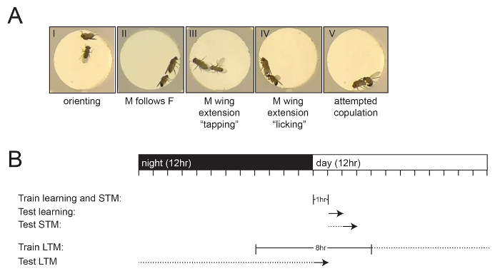
Figure 1: Determination of the Courtship Index and Experimental Overview. (A) Images showing stereotypical male courtship behavior towards a female fly. Different stages of courtship behavior are shown: orientation (I), following (II), wing vibration (extension) and tapping (III), licking (IV), and attempted copulation (V). (B) Schematic overview of training and testing times relative to the incubator light cycle, marked in hours. Training times are indicated with bars, resting periods for STM and LTM are indicated with a dashed line, and the testing start point is indicated as an arrow. Note that the testing time for LTM is the day after after training. Please click here to view a larger version of this figure.

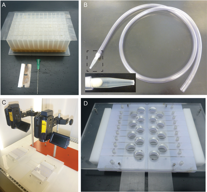
Figure 2: Equipment used for the Drosophila Courtship Conditioning Assay. (A) The housing block is a flat, bottom block with 500 µL of powerfood per well. It is sealed with a qPCR adhesive film with at least 4 holes per well that were created using a syringe needle with a 0.8 mm diameter. Individual rows are cut lengthwise into strips using a razor blade to allow opening and closing. (B) The aspirator is required for the gentle transfer of male and female flies without the use of anesthesia. The inset shows the tip of the aspirator, closed with a piece of cotton to keep the flies within the tip. (C) Setup of a two-camera system for the simultaneous recording of two courtship chambers. (D) A courtship chamber with 18 arenas. Sliding entry holes are used to place the flies in the arenas. The white dividers can be simultaneously opened to initiate interaction between the males and females. Please click here to view a larger version of this figure.

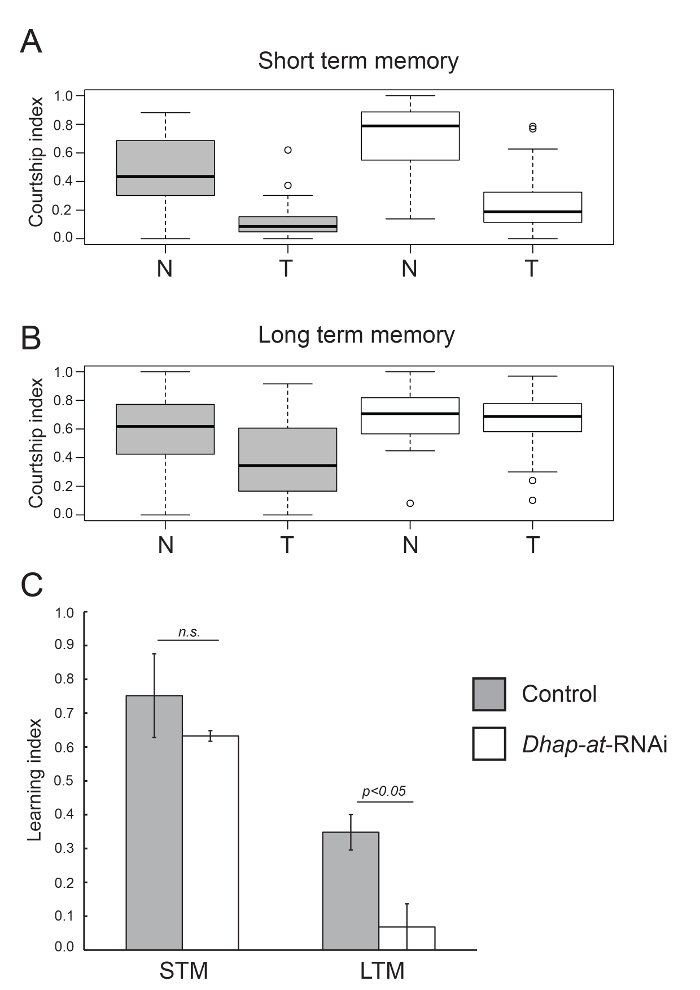
Figure 3: Analysis of STM and LTM in Control and Dhap-at Knockdown Flies. (A-B) Boxplots showing the distribution of CI values for naïve (N) and trained (T) flies of the control (gray) and Dhap-at knockdown (white) genotypes tested for STM (A) and LTM (B). (C) Corresponding LI values for control and Dhap-at knockdown flies tested for STM and LTM. Differences in LI between control and knockdown genotypes were compared using a randomization test (10,000 bootstrap replicates). Error bars indicate the standard error of the mean derived from the LI values calculated on different test days. The genotypes are: w+, UAS-dcr2/+; P{KK108109}VIE-260B/+; and elav-Gal4/+ (Control) and w+, UAS-dcr2/+;P{KK101437}VIE-260B/+; and elav-Gal4/+ (Dhap-at-RNAi). Please click here to view a larger version of this figure.

	General	Collect	Train	Test
day -11	Start premated female collection cultures (step 1.3)
day -10	Start cultures for the collection of male test subjects (step 2.2)
day 1		rep. 1
day 2		rep. 2
day 3		rep. 3
day 4		rep. 4	rep. 1
day 5			rep. 2	rep. 1
day 6			rep. 3	rep. 2
day 7			rep. 4	rep. 3
day 8				rep. 4
day 9	Video data analysis and statistics (step 8)
rep = repeat

Table 1: Example Timeline for Testing LTM over Three Replicates on Individual Days.

	Learning	STM	LTM
Training time	1 h.	1 h.	8 h.
Resting time	0 h.	1 h.	~ 24 h.
start training	0 h. ALO	0 h. ALO	4 h. BLO
stop training	1 h. ALO	1 h. ALO	4 h. ALO
start test	1 h. ALO	2 h. ALO	0 h. ALO (next day)
ALO = after lights turn on, BLO = before lights turn on, STM = short term memory, LTM = long term memory

Table 2: Training Duration, Training Times, and Testing Times for Learning, STM, and LTM.

Genotype	Learning condition	CI naive	CI trained	LI	LI difference	Lower limit (95% conficence interval)	Upper limit (95% conficence interval)	p-value
Control	STM	0.467	0.116	0.752	NA	NA	NA	NA
Dhap-at-RNAi	STM	0.699	0.257	0.633	0.119	-0.030	0.265	0.116
Control	LTM	0.590	0.384	0.348	NA	NA	NA	NA
Dhap-at-RNAi	LTM	0.697	0.650	0.068	0.280	0.103	0.446	0.003

Table 3: Statistical Data Produced from the Analearn Script.
Statistical data produced from the analearn script. The output file of the bootstrapping R-script containing the genotype, learning condition (i.e., learning, STM, or LTM), mean CI naïve, mean CI trained, LI, difference between LI of the control compared to experimental condition (LI dif), the lower limit (LL) and upper limit (UL) of the 95% confidence interval of LI dif, and the p-value indicating the probability that there is no significant difference.

		Control			Dhap-at-RNAi
		Average CI naïve	Average CI trained	LI	Average CI naïve	Average CI trained	LI
STM	Day 1	0.300	0.125	0.584	0.679	0.239	0.648
	Day 2	0.634	0.107	0.831	0.720	0.276	0.617
	All Days	0.467	0.116	0.752	0.699	0.257	0.633
LTM	Day 1	0.590	0.441	0.252	0.630	0.646	-0.027
	Day 2	0.640	0.363	0.432	0.709	0.710	-0.002
	Day 3	0.547	0.349	0.363	0.738	0.598	0.190
	All Days	0.590	0.384	0.348	0.697	0.650	0.068

Table 4: CI and LI Values Obtained on Separate Testing Days.

“naivelevel” determines the text that will identify naïve values for each genotype. The default is “N,” but this can be changed into any other alphanumerical text.

“refmutation” is set to “NA” (not applicable) by default, but can be changed to the name of the control or the genotype in order to perform statistical comparisons.  This will cause the script to automatically select the control genotype.

"datname” refers to the name of the data file and can be specified in this argument instead of the default file selection.

"header” can be used to indicate whether or not the data file contains column headers.  The default is “TRUE,” but a file with no headers can be used when this argument is changed to “FALSE.”

"seed” initializes the random number generator. This is set by default to “NA” and ensures a random number each time the script is used.  By design, a bootstrap analysis will give slightly different results each time it is run, even when using the same data file.  When the seed is specified by any integer number larger than zero, the same set of random bootstrap samples is obtained.

"writeoutput” can be set to “TRUE” or “FALSE” in order to determine whether an output file will be generated. The default is “TRUE.”

Table 5: Arguments used in the Analearn Function that Can Alter the Default Settings of the Function to Adjust the Parameters of the Bootstrapping

Supplemental File S1: Building plan of a courtship chamber. The file can be opened with any application that allows .stp extensions (CAD-files). Please click here to download this file.

Supplemental File S2: Example of an Input File for the Analearn Script. Please click here to download this file.

Supplemental File S3: The Analearn.R Acript. The file can be opened with R-studio¹⁸. Please click here to download this file.

Discussion

The courtship conditioning assay is a classic paradigm for the analysis of learning and memory in Drosophila. The protocol presented here follows the general methodology described previously^6,7,8,9 but includes unique aspects such as practical guidelines, specialized equipment, and a data analysis script^9,12 for randomization tests. Using this protocol, it is possible to analyze large numbers of flies in parallel using 96-well flat-bottom blocks (Figure 2A) to collect and train males. The blocks are sealed with PCR adhesive film, which makes the flies easily accessible when required. Additionally, the unique courtship chambers described here allow for the simultaneous pairing of 18 male-female pairs in a nearly two-dimensional space that is optimal for video analysis. The custom-designed courtship chambers are easy to use, and a building plan is provided (File S1, Figure 2D). This protocol, from the establishment of the cultures used to collect test subjects to the acquisition of video data, takes approximately 20 days (Table 1). Additional time is required for the analysis of video data. In our experience, the STM assay is extremely robust. The LTM assay is also quite robust, but it is more sensitive to confounding environmental variables and therefore can be more difficult to master.

Animal behavior can be quite variable. Therefore, critical steps in the protocol must be performed with care to reduce this variance. First, gentle use of the aspirator (Figure 2B) will reduce the stress that can be imposed by rough handling or by blowing out too strongly. A suggested method of transferring individual flies out of the aspirator is by using negative geotaxis. As flies tend to walk up, one can simply point the tip of the aspirator up; just before the fly reaches the tip, a gentle blow is sufficient to let the fly out. Additionally, to let the males into the courtship chambers before testing, a blow is often not necessary.

Another important step is the collection and generation of male test subjects. All males must be collected when they are very young and socially naïve. This can be achieved by frequent collection during the peak periods of eclosion (step 5.2). If males are not collected in this tight timeframe, they can have early social interactions, which may result in poor learning or high variability in CI. Another factor of male test subjects that should be assessed is the genetic background. Different genetic backgrounds will exhibit different levels of naïve courtship and may also differ in general activity or locomotor ability. When comparing multiple genotypes, care should be taken with regard to genetic background in order to avoid these confounding factors that may influence LI scores. Additionally, the distribution of CI data should be carefully assessed. CI data can be both parametric and non-parametric, depending on the genotype or other environmental factors. In some cases, if the distribution of CI is dramatically skewed away from a normal distribution, it may be better to use the median CI rather than the mean for the calculation of LIs. However, in our experience, the use of median or mean CI does not make a difference in the statistical interpretation of the data, and the use of the mean CI is the common practice in the literature.

For successful courtship conditioning, the active rejection of male courtship attempts by premated females is crucial during the training period. It is important to ensure that the premated females used in this assay have been efficiently mated and are thus not allowing copulation. This premating is established in the mating vials prepared in step 4, where male and females flies are housed together for 4 days (Table 1). Subsequently, mating can be monitored by regular examination of testing videos and by observing male-female pairs during training. If mating does occur, there are several measures that can be taken during the preparation of premated females. First, premated females should be reared under optimal breeding conditions. Vials can be supplemented with yeast paste and a folded filter paper to increase potential mating surfaces. The incubation of flies under the conditions described here has produced robust premated females in the past, but this may vary in different labs and with the use of different genetic strains. Therefore, it may be necessary to optimize the generation of premated females by varying the incubation time and conditions.

Quantification of courtship behavior is another critical step in this protocol. This can be done manually or automatically using specialized software programs⁹. Automated quantification is fast and, in principle, unbiased. Several programs have been published^21,22,23; however, they are not straightforward to use, often requiring specialized video formats and advanced computational skills. Manual quantification is easy and accurate, but it is highly labor intensive and subject to individual variability and bias. It is important to emphasize that this protocol does not address the requirements for video formatting that are potentially required for the automated quantification of CIs. For manual quantification, use any simple video recording device that has the potential to produce a video of sufficient quality to accurately observe courtship behavior. For automated quantification, there will likely be different requirements depending on the software used, and users should investigate this thoroughly if automated quantification is desired.

In combination with the extensive tools that are available for the genetic manipulation of flies, the courtship conditioning assay provides a robust readout that can be used to dissect molecular mechanisms and neuronal networks involved in learning and memory.

Materials

List of materials used in this article

Name	Company	Catalog Number	Comments
P{KK101437}VIE-260B	VDRC	101437	Dhat-at-RNAi in 60100 background
P{KK108109}VIE-260B	-	-	Control-RNAi in 60100 background (gift from K. Keleman)
w+, UAS-dcr2/yhh;;elav-Gal4 (III)	-	-	panneuronal driver line
Containers for plant tissue culture	VWR	960177	175 mL plastic vials
Folded filters	Whatman	10311643	Filter paper to enlarge area flies can pupate on
Flat-bottom blocks (96-wells)	Qiagen	19579	Used for housing blocks
MicroAmp Clear Adhesive Film	Applied Biosystems	4306311	PCR adhesive film as lid on flat-bottom blocks
Razor blade	-	-	Any sharp will do
Needle	-	-	0.8 mm diameter
Aspirator	-	-	Cut a 1mL pipet tip with scissors in order to have two pieces. The narrow tip of the pipettip is placed as fly entrance in a ~80 cm flexible hose. To prevent a fly from getting in the hose, a normal piece of cotton or small mesh gaze is placed in between the tip and the hose. The other half of the pipettip can be used as mouth piece at the end of the hose.
Courtship chambers	-	-	file S1 can be opened with indicated CAD software
Camcorder	Sony	-	camera specification: >4M pixels, full HD. For manual quantification, any simple video recording device has the potential to produce a video of sufficient quality to observe courtship behavior accurately. For automated quantification, there will likely be different requirements depending on the software to be used, and users should investigate this thoroughly if automated quantification is desired.
Name	Company	Catalog Number	Comments
power food
Agar	Sigma	A7002
Yeast	Bruggeman	-
Yeast extract	MP biomedicals	0210330391
Peptone	Sigma	P6838
Sucrose	Sigma	S9378
Glucose	Sigma	G7021
MgSO4	Sigma	M2643
CaCl2	Merck	1023780500
Methylparabene (CAUTION)	Sigma	H5501
Propionic acid (CAUTION)	Sigma	P1386
Demineralized water	-
Yeast paste	-		yeast grains and water mixture in a 1:1 ratio
Name	Company	Catalog Number	Comments
normal food
Agar	MP biomedicals	215017890
Yeast	bruggeman	-
Corn flour	de Molen	-
Sugar	de Molen	-
Methylparabene (CAUTION)	Sigma	H5501
Propionic acid (CAUTION)	Sigma	P1386
Demineralized water	-

References

- Quinn, W. G., Harris, W. A., Benzer, S. Conditioned behavior in Drosophila melanogaster. Proc. Natl. Acad. Sci. USA. 71, 708-712 (1974).
- Livingstone, M. S., Sziber, P. P., Quinn, W. G. Loss of calcium/calmodulin responsiveness in adenylate cyclase of rutabaga, a Drosophila learning mutant. Cell. 37, 205-215 (1984).
- Quinn, W. G., Sziber, P. P., Booker, R. The Drosophila memory mutant amnesiac. Nature. 277, 212-214 (1979).
- Dudai, Y., Jan, Y. N., Byers, D., Quinn, W. G., Benzer, S. dunce, a mutant of Drosophila deficient in learning. Proc. Natl. Acad. Sci. USA. 73, 1684-1688 (1976).
- Dubnau, J., Tully, T. Gene discovery in Drosophila: new insights for learning and memory. Annu. Rev. Neurosci. 21, 407-444 (1998).
- Siegel, R. W., Hall, J. C. Conditioned responses in courtship behavior of normal and mutant Drosophila. Proc. Natl. Acad. Sci. USA. 76, 3430-3434 (1979).
- Kamyshev, N. G., Iliadi, K. G., Bragina, J. V. Drosophila conditioned courtship: two ways of testing memory. Learning & memory. 6, 1-20 (1999).
- McBride, S. M., et al. Mushroom body ablation impairs short-term memory and long-term memory of courtship conditioning in Drosophila melanogaster. Neuron. 24, 967-977 (1999).
- Keleman, K., Kruttner, S., Alenius, M., Dickson, B. J. Function of the Drosophila CPEB protein Orb2 in long-term courtship memory. Nature Neurosci. 10, 1587-1593 (2007).
- Hall, J. C. The mating of a fly. Science. 264, 1702-1714 (1994).
- Keleman, K., et al. Dopamine neurons modulate pheromone responses in Drosophila courtship learning. Nature. 489, 145-149 (2012).
- Kramer, J. M., et al. Epigenetic regulation of learning and memory by Drosophila EHMT/G9a. PLoS Biol. 9. 9, e1000569(2011).
- Ishimoto, H., Sakai, T., Kitamoto, T. Ecdysone signaling regulates the formation of long-term courtship memory in adult Drosophila melanogaster. Proc. Natl. Acad. Sci. USA. 106, 6381-6386 (2009).
- Kochinke, K., et al. Systematic Phenomics Analysis Deconvolutes Genes Mutated in Intellectual Disability into Biologically Coherent Modules. Am. J. Hum. Genet. 98, 149-164 (2016).
- Buchert, R., et al. A peroxisomal disorder of severe intellectual disability, epilepsy, and cataracts due to fatty acyl-CoA reductase 1 deficiency. Am. J. Hum. Genet. 95, 602-610 (2014).
- JoVE Science Education Database. Essentials of Biology 1: yeast, Drosophila and C. elegans. Drosophila Maintenance. JoVE. , Cambridge, MA. (2017).
- JoVE Science Education Database. Essentials of Biology 1: yeast, Drosophila and C. elegans. An Introduction to Drosophila melanogaster. JoVE. , Cambridge, MA. (2017).
- R Core Team. R: A Language and Environment for Statistical Computing. R Foundation for Statistical Computing. , Vienna (Austria). (2016).
- Stepien, B. K., et al. RNA-binding profiles of Drosophila CPEB proteins Orb and Orb2). Proc. Natl. Acad. Sci. USA. 113, E7030-E7038 (2016).
- Basu, D. Randomization Analysis of Experimental Data: The Fisher Randomization Test. J Am Stat Assoc. 75, 575-582 (1980).
- Dankert, H., Wang, L., Hoopfer, E. D., Anderson, D. J., Perona, P. Automated monitoring and analysis of social behavior in Drosophila. Nat Methods. 6, 297-303 (2009).
- Reza, M. A., et al. Automated analysis of courtship suppression learning and memory in Drosophila melanogaster. Fly. 7, 105-111 (2013).
- Schneider, J., Levine, J. D. Automated identification of social interaction criteria in Drosophila melanogaster. Biol. Lett. 10, 20140749(2014).
Reprints and Permissions