Quelle: Dominique R. Bollino1, Eric A. Legenzov2, Tonya J. Webb1
1 Department of Microbiology and Immunology, University of Maryland School of Medicine and the Marlene and Stewart Greenebaum Comprehensive Cancer Center, Baltimore, Maryland 21201
2 Center for Biomedical Engineering and Technology, University of Maryland School of Medicine, Baltimore, Maryland 21201
Die konfokale Fluoreszenzmikroskopie ist eine bildgebende Technik, die eine höhere optische Auflösung im Vergleich zur herkömmlichen “Weitfeld”-Epifluoreszenzmikroskopie ermöglicht. Konfokale Mikroskope sind in der Lage, eine verbesserte x-y optische Auflösung durch “Laserscanning” zu erreichen – typischerweise eine Reihe von spannungsgesteuerten Spiegeln (Galvanometer oder “Galvo”-Spiegel), die Laserbeleuchtung auf jedes Pixel der Probe zu einem Zeitpunkt leiten. Noch wichtiger ist, dass konfokale Mikroskope eine überlegene z-axiale Auflösung erreichen, indem sie ein Loch verwenden, um aus fokussiertem Licht zu entfernen, das von Orten stammt, die sich nicht in der zu scannenden Z-Ebene befinden, wodurch der Detektor Daten von einer bestimmten Z-Ebene sammeln kann. Durch die hohe Z-Auflösung, die in der konfokalen Mikroskopie erreichbar ist, ist es möglich, Bilder aus einer Reihe von Z-Ebenen (auch z-stack genannt) zu sammeln und ein 3D-Bild durch Software zu konstruieren.
Bevor Sie den Mechanismus eines konfokalen Mikroskops diskutieren, ist es wichtig zu überlegen, wie eine Probe mit Licht interagiert. Licht besteht aus Photonen, Paketen elektromagnetischer Energie. Ein Photon, das auf eine biologische Probe einwirkt, kann mit den Molekülen interagieren, die die Probe umfassen, auf eine von vier Arten: 1) das Photon interagiert nicht und durchläuft die Probe; 2) das Photon reflektiert/gestreut wird; 3) das Photon wird von einem Molekül absorbiert und die absorbierte Energie wird als Wärme durch Prozesse freigesetzt, die kollektiv als nicht-radioativer Zerfall bekannt sind; und 4) das Photon wird absorbiert und die Energie wird dann schnell als sekundäres Photon durch den als Fluoreszenz bekannten Prozess übersendet. Ein Molekül, dessen Struktur die Fluoreszenzemission zulässt, wird als Fluorophor bezeichnet. Die meisten biologischen Proben enthalten vernachlässigbare endogene Fluorophore; daher müssen exogene Fluorophore verwendet werden, um Merkmale hervorzuheben, die für die Probe von Interesse sind. Während der Fluoreszenzmikroskopie wird die Probe mit Licht der entsprechenden Wellenlänge für die Absorption durch das Fluorophor beleuchtet. Bei der Aufnahme eines Photons wird ein Fluorophor als “erregt” bezeichnet und der Absorptionsprozess wird als “Erregung” bezeichnet. Wenn ein Fluorophor Energie in Form eines Photons aufgibt, wird das Verfahren als “Emission” bezeichnet, und das emittierte Photon wird Fluoreszenz genannt.
Der Lichtstrahl, der zur Erregung eines Fluorophors verwendet wird, wird durch die Objektivlinse eines Mikroskops fokussiert und konvergiert an einem “Fokalpunkt”, wo er maximal fokussiert ist. Jenseits des Brennpunkts weicht das Licht wieder ab. Die ein- und austretenden Balken können als kegelndes Kegelpaar visualisiert werden, das sich am Brennpunkt berührt (siehe Abbildung 1, linkes Panel). Das Phänomen der Beugung setzt eine Grenze, wie eng ein Lichtstrahl fokussiert werden kann – der Strahl konzentriert sich tatsächlich auf einen Punkt von endlicher Größe. Zwei Faktoren bestimmen die Größe des Brennpunkts: 1) die Wellenlänge des Lichts und 2) die Lichtaufnahmefähigkeit der Objektivlinse, die sich durch ihre numerische Blende (NA)auszeichnet. Der brennpunktige “Spot” erstreckt sich nicht nur in der x-y-Ebene, sondern auch in z-Richtung und ist in Wirklichkeit ein Brennvolumen. Die Abmessungen dieses Brennvolumens definieren die maximale Auflösung, die durch optische Bildgebung erreicht wird. Obwohl die Anzahl der Photonen innerhalb des Brennvolumens am größten ist, enthalten die konischen Lichtpfade oberhalb und unterhalb des Fokus auch eine geringere Dichte von Photonen. Jedes Fluorophor im Lichtpfad kann so angeregt werden. In der konventionellen (Weitfeld-)Epifluoreszenzmikroskopie tragen die Emissionen von Fluorophoren oberhalb und unterhalb der Brennebene zur außerfokussierenden Fluoreszenz bei (ein “hazy background”), was die Bildauflösung und den Kontrast reduziert, wie in Abbildung 1 der rote Würfel, der die Fluorophoremission über der Brennebene (roter Stern) darstellt, die zu einer nicht fokussierten Fluoreszenz führt (oben rechts). Dieses Problem wird in der konfokalen Mikroskopie durch die Verwendung eines Lochs gemildert. (Abbildung 2, unten rechts). Wie in Abbildung 3 dargestellt, ermöglicht das Loch Emissionen, die vom Brennpunkt ausgehen, den Detektor (links) zu erreichen, während die nicht fokussierte Fluoreszenz (rechts) am Erreichen des Detektors gehindert wird, wodurch sowohl die Auflösung als auch der Kontrast verbessert werden.
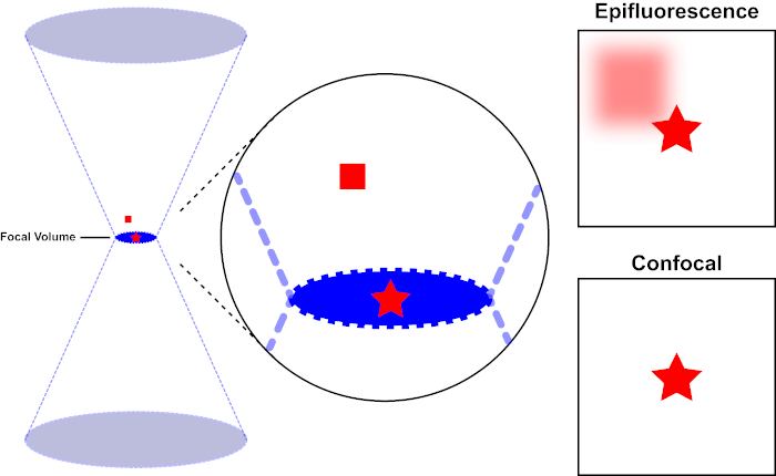
Abbildung 1. Optische Auflösung der Epifluoreszenz versus konfokale Mikroskopie. Bitte klicken Sie hier, um eine größere Version dieser Abbildung anzuzeigen.
Der Lichtstrahl, der zur Anregung eines Fluorophors verwendet wird, wird durch die Objektivlinse eines Mikroskops fokussiert und konvergiert bei einem Brennvolumen und weicht dann ab (links). Der rote Stern stellt die Brennebene einer Probe dar, die abgebildet wird, während das rote Quadrat die Fluorophoremission über der Brennebene darstellt. Bei der Aufnahme eines Bildes dieser Probe mit einem Epifluoreszenzmikroskop wird die Emission des roten Quadrats a-fokus sichtbar und trägt zu einem “hazy background” (oben rechts) bei. Konfokale Mikroskope haben ein Loch, das die Erkennung von Licht verhindert, das außerhalb der Brennebene emittiert wird, wodurch der “hazy background” (unten rechts) eliminiert wird.
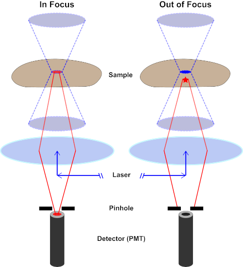
Abbildung 2. Locheffekt in der konfokalen Mikroskopie. Bitte klicken Sie hier, um eine größere Version dieser Abbildung anzuzeigen.
Obwohl die höchste Intensität des Anregungslichts am Brennpunkt der Linse (links, rot oval) liegt, erhalten andere Teile der Probe, die sich nicht im Brennpunkt befindet (rechts, roter Stern), Licht und Fluoreszenz. Um zu verhindern, dass Licht aus diesen nicht fokussierten Bereichen zum Detektor gelangt, befindet sich ein Bildschirm mit einem Loch vor dem Detektor. Nur das von der Brennebene emittende Infokuslicht (links) kann durch das Loch reisen und den Detektor erreichen. Das nicht fokussierte Licht (rechts) wird mit dem Loch blockiert und erreicht den Detektor nicht.
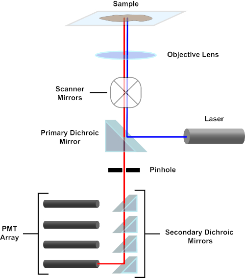
Abbildung 3. Hauptkomponenten eines konfokalen Laserscanmikroskops. Bitte klicken Sie hier, um eine größere Version dieser Abbildung anzuzeigen.
Der Einfachheit halber wird sich die mechanistische Beschreibung eines konfokalen Mikroskops auf die des Nikon Eclipse Ti A1R beschränken. Obwohl es geringfügige technische Unterschiede zwischen verschiedenen konfokalen Mikroskopen geben kann, dient das A1R sowohl als gutes Modell für die Beschreibung der konfokalen Mikroskopfunktion. Der anregungslichtstrahl, der durch eine Reihe von Diodenlasern erzeugt wird, wird vom primären dichroitischen Spiegel in das Objektiv reflektiert, der das Licht auf die abgebildete Probe fokussiert. Der primäre dichroitische Spiegel reflektiert selektiv das Anregungslicht und lässt gleichzeitig Licht bei anderen Wellenlängen passieren. Das Licht trifft dann auf die Scanspiegel, die den Lichtstrahl x-y x-y über die Probe fegen und gleichzeitig ein einzelnes (x,y) Pixel beleuchten. Fluoreszenz, die von Fluorophoren am beleuchteten Pixel emittiert wird, wird von der Objektivlinse erfasst und durchläuft den primären dichroitischen Spiegel, um eine Reihe von Photomultiplierröhren (PMTs) zu erreichen. Sekundäre dichroitische Spiegel leiten das Emissionslicht auf das entsprechende PMT. Von der Probe in das Objektiv gestreutes Anregungslicht wird durch den primären dichroitischen Spiegel zurück zur Probe reflektiert und somit am Eindringen in den Nachweis gehindert. Lichtpfad und erreichen die PMTs (siehe Abbildung 3). Dadurch kann die relativ schwache Fluoreszenz ohne Kontamination durch Licht quantifiziert werden, das vom Anregungslichtstrahl gestreut wird, der typischerweise um Größenordnungen intensiver ist als die Fluoreszenz. Da das Loch Licht von außerhalb des Brennvolumens blockiert, kommt das Licht, das beim Detektor ankommt, von einer schmalen, ausgewählten Z-Ebene. Daher können Bilder aus einer Reihe benachbarter z-Ebenengesammelt werden; diese Bilderserie wird oft als “Z-Stack” bezeichnet. Mit der entsprechenden Software kann ein z-Stackverarbeitet werden, um ein 3D-Bild der Probe zu erzeugen. Ein besonderer Vorteil der konfokalen Mikroskopie ist die Fähigkeit, die subzelluläre Lokalisation der Färbung zu unterscheiden. Zum Beispiel die Unterscheidung zwischen Membranfärbung und intrazellulärer Färbung, die bei der konventionellen Epifluoreszenzmikroskopie (1, 2, 3) sehr anspruchsvoll ist.
Die Probenvorbereitung ist eine wichtige Facette der konfokalen Bildgebung. Eine Stärke der optischen Mikroskopie-Techniken ist die Flexibilität, lebende oder feste Zellen abzubilden. Beim Versuch, 3D-Bilder zu erzeugen, ist die Verwendung fester Zellen aufgrund der Anzahl der Bilder, die für einen Z-Stack erworben werden müssen, der Schwierigkeit, die Zellgesundheit zu erhalten, und der Bewegung von lebenden Zellen und ihren Organellen typisch. Das Verfahren zur Fixierung und Färbung von Zellen zur konfokalen Fluoreszenz ähnelt dem, das konventionell bei der Immunfluoreszenz verwendet wird. Nach der Kultur in Kammerrutschen oder auf Abdeckungen werden Zellen mit Paraformaldehyd fixiert, um die zelluläre Morphologie zu erhalten. Die unspezifische Antikörperbindung wird mit Rinderserumalbumin, Milch oder normalem Serum blockiert. Um die Spezifität der sekundären Antikörper aufrechtzuerhalten, sollte die verwendete Lösung nicht von derselben Art stammen, bei der die primären Antikörper erzeugt wurden. Die Zellen werden mit primären Antikörpern inkubiert, die das Antigen von Interesse binden. Bei der Kennzeichnung mehrerer zellulärer Ziele müssen die primären Antikörper jeweils von einer anderen Spezies abgeleitet werden. Antikörper, die ein Antigen kennzeichnen, werden dann durch fluorophorkonjugierte sekundäre Antikörper gebunden. Fluorophorkonjugierte Sekundärantikörper sollten so ausgewählt werden, dass sie mit den Wellenlängen der Lasererregung im konfokalen Mikroskop kompatibel sind. Bei der Visualisierung mehrerer Antigene sollten sich die Anregungs-/Emissionsspektren der Fluorophore so weit unterscheiden, dass ihre Signale durch mikroskopische Analysen diskriminiert werden können. Die gebeizte Probe wird dann zur Bildgebung auf einem Dia montiert. Ein Montagemedium wird verwendet, um Photobleichungen und Probenaustrocknung zu verhindern. Auf Wunsch kann ein Montagemedium verwendet werden, das einen nuklearen Gegenfleck enthält (z.B. DAPI oder Hoechst) (4).
Im folgenden Protokoll wurden Maus-Fibroblasten, die auf CD1d (LCD1) transfiziert wurden, mit Antikörpern gefärbt, die CD1d und CD107a (LAMP-1) erkennen. CD1d ist ein wichtiger Histokompatibilitätskomplex 1 (MHC 1)-ähnlicher Rezeptor, der auf der Oberfläche von Antigen-Präsentierenden Zellen vorhanden ist, die Lipidantigene darstellen. LAMP-1 (lysosomal assoziiertes Membranprotein-1) ist ein Transmembranprotein, das hauptsächlich in lysosomalen Membranen vorkommt. Für die richtige Antigen-Präsentation wird CD1d durch das niedrige pH-Lysosomalfach geschmuggelt, so dass LAMP-1 als Marker des lysosomalen Fachs für dieses Protokoll verwendet wird. Durch die Untersuchung der LCD1-Zellen mit Anti-CD1d und Anti-LAMP-1, die in verschiedenen Arten hergestellt wurden, können sekundäre Antikörper mit einzigartigen Fluorophoren verwendet werden, um die Lokalisation jedes Proteins in der Zelle zu bestimmen und ob CD1d in der LAMP-1-positiven lysosomalen Fächern.
In this experiment, mouse fibroblasts expressing the surface glycoprotein gene CD1d were fixed, immunostained and imaged on a confocal microscope. A representative image obtained using the above protocol is shown in Figure 4. In the top panel of A, single-channel images showing the staining pattern of each individual target are presented. These images comprise a single section (slice) of the z-stack captured. The right panel shows DAPI staining of nuclei of the cells. The center panels show CD1d stained in red and LAMP-1, a lysosomal marker, stained in green. The left panel is a composite image where the three different channels are merged. The appearance of yellow results from overlap of the red and green channels, and indicates an area where CD1d and LAMP-1 are co-localized. The results of the staining confirm that CD1d is localized in the LAMP-1+ endosomal compartments. There are also areas where only one color is present, which indicates the presence of CD1d or LAMP-1 without co-localization. The bottom panel of A shows a 3D rendering of the cells constructed from images captured in the z-stack.
Panel B shows a slice out of the z-stack at 100x magnification demonstrating the expression patterns of these two proteins in greater detail. The pink outlined box on the right side of the image displays the cross section of the x-coordinate designated by the pink line in the image, which represents the side view at the pink line. Similarly, the blue outlined box on the bottom of the image shows the cross section of the y-coordinate designated by the blue line in the image, which represents the front view at the blue line. The 3D rendering of the z-stack image enables users to view the image in 3D, visualizing all the x, y and z planes.

Figure 4: Staining of CD1d and LAMP1. Please click here to view a larger version of this figure.
A, top panel: LCD1 cells were fixed, permeabilized and stained with antibodies to CD1d (red) and LAMP-1 (green, a marker of the lysosomal compartment). DAPI (blue, was used to visualize the nucleus). The merge (left panel) shows that CD1d is localized in the LAMP-1 positive late endosomal/lysosomal compartment (yellow).
A, bottom panel: 3D rendering of the same cells in top panel. Images were acquired using a 40x oil-immersion objective on the Nikon Eclipse Ti, using the NIS Elements Advanced Research software.
B: 100x image of LCD1d cells stained as in A, with stack information for a particular y-coordinate (denoted by the blue line) on the bottom of the image (blue box). The stack information for a particular x-coordinate (denoted by the pink line) is shown on the right side of the image (pink box).
Confocal fluorescent staining is a relatively simple procedure that results in extremely high-quality images of specimens that are prepared in a similar way as for conventional fluorescence microscopy. In brief, samples are fixed, permeabilized, then blocked. Primary antibodies against a protein or proteins of interest are allowed to bind, then fluorophore-conjugated secondary antibodies are used to visualize the staining. Confocal fluorescence microscopy has applications in many areas of research. For example, by staining for markers of sub-cellular organelles along with a protein of interest, confocal microscopy can be used to determine the subcellular locations of diverse proteins. Compared to conventional fluorescence microscopy, confocal imaging can more effectively distinguish between cell surface and intracellular location of a protein. In addition, confocal imaging can also be used to determine whether two proteins co-localize within the cell. Although not outlined in this protocol, confocal fluorescence microscopy also can be performed on live cells to detect dynamic changes.

Video 1: Video created in NIS Elements Advanced Research software, highlighting the ability to move through the 3D rendering of the images. Please click here to view this video (Right click to download).