Methods for Measuring the Orientation and Rotation Rate of 3D-printed Particles in Turbulence

Summary

We use 3D printing to fabricate anisotropic particles in the shapes of jacks, crosses, tetrads, and triads, whose alignments and rotations in turbulent fluid flow can be measured from multiple simultaneous video images.

Abstract

Experimental methods are presented for measuring the rotational and translational motion of anisotropic particles in turbulent fluid flows. 3D printing technology is used to fabricate particles with slender arms connected at a common center. Shapes explored are crosses (two perpendicular rods), jacks (three perpendicular rods), triads (three rods in triangular planar symmetry), and tetrads (four arms in tetrahedral symmetry). Methods for producing on the order of 10,000 fluorescently dyed particles are described. Time-resolved measurements of their orientation and solid-body rotation rate are obtained from four synchronized videos of their motion in a turbulent flow between oscillating grids with R_λ = 91. In this relatively low-Reynolds number flow, the advected particles are small enough that they approximate ellipsoidal tracer particles. We present results of time-resolved 3D trajectories of position and orientation of the particles as well as measurements of their rotation rates.

Introduction

In a recent publication, we introduced the use of particles made from multiple slender arms for measuring rotational motion of particles in turbulence¹. These particles can be fabricated using 3D printers, and it is possible to accurately measure their position, orientation, and rotation rate using multiple cameras. Using tools from slender body theory, it can be shown that these particles have corresponding effective ellipsoids², and the rotational motions of these particles are identical to those of their respective effective ellipsoids. Particles with symmetric arms of equal length rotate like spheres. One such particle is a jack, which has three mutually perpendicular arms attached at its center. Adjusting the relative lengths of the arms of a jack can form a particle equivalent to any tri-axial ellipsoid. If the length of one arm is set equal to zero, this creates a cross, whose equivalent ellipsoid is a disk. Particles made of slender arms take up a small fraction of the solid volume of their solid ellipsoidal counterparts. As a result, they sediment more slowly, making them easier to density match. This allows the study of much larger particles than is convenient with solid ellipsoidal particles. Additionally, imaging can be performed at much higher particle concentrations because the particles block a smaller fraction of the light from other particles.

In this paper, methods for fabrication and tracking of 3D-printed particles are documented. Tools for tracking the translational motion of spherical particles from particle positions as seen by multiple cameras have been developed by several groups^3,4. Parsa et al.⁵ extended this approach to track rods using the position and orientation of the rods seen by multiple cameras. Here, we present methods for fabricating particles of a wide variety of shapes and reconstructing their 3D orientations. This offers the possibility to extend 3D tracking of particles with complex shapes to a wide range of new applications.

This technique has great potential for further development because of the wide range of particle shapes that can be designed. Many of these shapes have direct applications in environmental flows, where plankton, seeds, and ice crystals come in a vast array of shapes. Connections between particle rotations and fundamental small-scale properties of turbulent flows⁶ suggest that study of rotations of these particles provides new ways to look at the turbulent cascade process.

Protocol

1. Fabrication of Particles

1. Use a 3D Computer Aided Drafting program to create particle models. Export one file per model in a file format that can be processed by the 3D printer used.
   1. Use the Circle command to draw a circle with a diameter of 0.3 mm. Use the Extrude function to make a cylinder with a length of 3 mm.
   2. Make a cross with two orthogonal cylinders with a common center; make a jack with three mutually orthogonal cylinders with a common center; make a tetrad with four cylinders sharing a common end at 109.5° angles to one another; make a triad with three cylinders in a plane sharing a common end at 120° angles to one another.
   3. To tilt cylinders (hereafter called "arms" of the particles) with respect to one another, use the Rotate 3D command to draw a line across the diameter of the circle at one of its ends and then enter the desired angle of rotation.
   4. Use the Union command to join the different arms together into a single watertight object.
   5. Use Rotate 3D again to tilt the object so that no arms are along the vertical or horizontal axes, because arms that lie along these axes tend to have defects, break off more easily, or flatten out.
   6. Export each object in a separate file in a format that can be used by 3D printers.
2. Order approximately 10,000 particles of each type from a commercial source that specializes in additive manufacturing or print them at an available facility. Particles should be printed on a polymer extrusion printer that uses a support matrix of a different material that can be dissolved away.
   1. Order the particles three weeks or more before experiments are planned because the arrangement and printing of so many particles is a slow process. Ensure that particles are printed on "high-resolution mode" because the particles are near the minimum feature size of many 3D printers and the arms will not be as symmetric and may break if printed at lower resolution.

2. Preparation of Particles 

1. Prepare a salt solution in which the particles are neutrally buoyant to minimize particles' arms bending while in storage and so that gravitational and buoyancy forces do not have to be accounted for in the analysis.
   1. Test average particle densities by immersing particles in solutions of water mixed with calcium chloride (CaCl₂) at densities around 1.20 g/cm³.
      1. To determine water density, first zero a scale while an empty 100 ml volumetric flask is on top of it. Take the flask off and fill it with water mixed with CaCl₂. Place the flask back atop the scale and divide the given mass by 100 ml.
         Note: Because 1 ml = 1 cm³, 1 g/ml = 1 g/cm³.
      2. Test particles at many different solution densities, ranging from 1.16 g/cm³ to 1.25 g/cm³, in roughly 0.01 g/cm³ increments. Test multiple particles at every density because not all particles will have the same density: in the same solution, some will sink, some will be neutrally buoyant, and some will float.
   2. Record at which density particles are, on average, neutrally buoyant after several hours.
      Note: The density found may be significantly different from the bulk density quoted by the particle manufacturers.
   3. Mix about 400 kg of CaCl₂ into approximately 1,600 L of water until the solution is at the density recorded in 2.1.1 - 2.1.2.
   4. Remove about 1 L of this mixed solution per particle type (jacks, tetrads, etc.) to be used for storage of particles. Hold each liter in a different container at room temperature. Store the remainder of the solution at room temperature in a large storage tank.

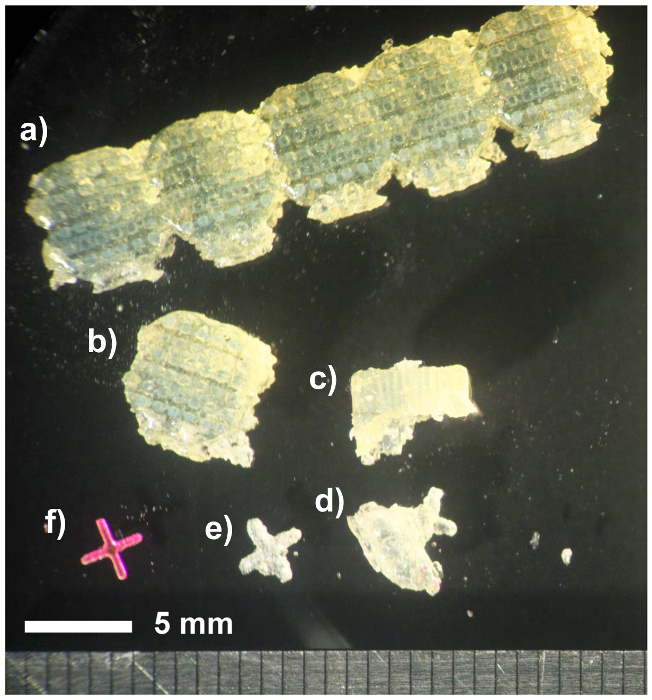
Figure 1. A jack at various stages of resin removal. a) The blocks of support resin that the particles arrive in. b) A single block separated from the rest. c-e) Multiple stages of resin removal done by hand. f) A single jack after the NaOH bath and Rhodamine-B dye. Please click here to view a larger version of this figure.

2. Manually loosen the support material in which the particles come encased by gently breaking the large pieces (~ 5 mm x 320 mm, part of which is shown in Figure 1a) into small sections (~5 mm x 5 mm, Figure 1b), then manually massage each section until much of the excess resin has come off (Figure 1c-e). Remove excess resin in this way to reduce the amount of the NaOH solution that will need to be created for steps 2.2.1 - 2.2.4.
   1. Place the remaining resin block in a 10% by mass sodium hydroxide (NaOH) solution immersed in an ultrasonic bath for one hour. The resin is a different material than the particles are, so the NaOH will remove the resin without permanently affecting the particles.
      CAREFUL: The solution is corrosive and will get hot while in the ultrasonic bath.
   2. Filter out particles.
      1. To filter particles, create a funnel using netting with 0.1016 cm x 0.13462 cm plastic holes. Hold the funnel over the container to be used for the disposal of the NaOH solution and slowly pour the solution through. Dispose of NaOH solution in accordance with environmental health and safety guidelines.
   3. Rinse particles gently with water before immersing in a new 10% by mass NaOH solution in an ultrasonic bath for another half hour.
   4. Filter out particles as in 2.2.2.1 and store in the density-matched solution separated in 2.1.4 while they harden. Handle the particles carefully because the NaOH solution temporarily softens them.
      Note: If particles are not stored in a density-matched solution, some arms may bend. Keeping them immersed in the density-matched solution for several hours also allows some voids in the plastic to fill with fluid.
3. Dye particles with Rhodamine-B mixed with water so that they fluoresce under the light emitted by a green laser.
   1. Prepare a 1 L solution of Rhodamine-B dye in water at a concentration of 0.5 g/L (afterward referred to as "dye").
      CAUTION: Toxic.
   2. Heat the dye to a temperature between 50 and 80 °C, depending on particle material. Use higher temperatures for harder plastics; using too high of a temperature will result in the arms bending.
   3. Put ~2,500 particles, enough to loosely fill ~25 ml in the density-matched storage solution, in the dye and keep all at 80 °C for two to three hours to allow the dye to absorb into the polymer. Remove particles once they are pink, like the one in Figure 1f.
      CAREFUL: The heat will soften the particles temporarily.
   4. Filter out particles and rinse them before storage in the designated solutions separated in 2.1.4. The particles will lose a small fraction of their dye, making the solution pink, but rinsing under the faucet helps prevent losing a detrimental amount of dye.
      Note: Average particle density will have changed due to dyeing, so test again as in 2.1.1-2.1.2 to find the new solution density at which particles are, on average, neutrally buoyant.
4. Change bulk CaCl₂ solution (from 2.1.3) density as needed. Repeat 2.1.4 and remove new volumes of density-matched solution. Dispose of former storage solutions, which will now have small amounts of Rhodamine-B dye in them, in accordance with environmental health and safety regulations.
5. Repeat 2.3.2-2.3.4 for successive sets of ~2,500 particles, storing all particles of the same shape in the same density-matched solutions created in 2.4, separated from particles of different shapes.
   Note: After about 5 repetitions of 2.3.2-2.3.4, the Rhodamine-B solution will no longer be a high enough concentration to effectively dye particles.
6. Dispose of the solution created in 2.3.1 in accordance with environmental health and safety regulations, then repeat 2.3.1 and create a new 0.5 g/L solution with which to dye particles.
7. Repeat 2.6 every 5 repetitions of 2.3.2-2.3.4.

3. Experimental and Optical Setup

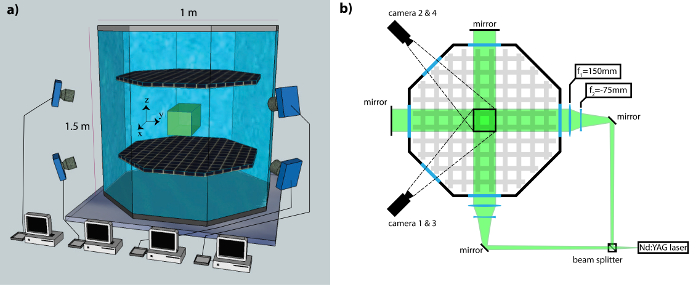
Figure 2. Experimental setup. In the octagonal flow between oscillating grids, a central viewing volume in the focus of the four video cameras is illuminated by a green Nd:YAG laser. a) Side view showing how the four cameras are arranged and connected to computers. Figure from ¹³. b) Top view showing laser, mirror, and lens configuration to achieve uniform illumination in the central volume. Please click here to view a larger version of this figure.

1. Prepare the cameras.
   1. Use cameras capable of at least 1 megapixel resolution at 450 frames per second.
   2. Arrange the cameras such that each camera is pointing at, and is focused on, the center of the viewing volume. Fewer cameras can be used, however shadowing of an arm of a particle by another arm limits the orientation measurement accuracy, and having fewer cameras makes experiments more susceptible to this effect. Using more than four cameras could likewise increase orientation measurement precision because it will reduce the chance of arms being shadowed on all cameras, which is a primary source of uncertainty.
   3. Position the cameras with large (~90°) angles between each pair subject to constraints of the apparatus. Place cameras as shown in Figure 2 to balance experimental access and the size of the angle between individual cameras. Minimize optical distortions by building viewing ports into the apparatus perpendicular to each camera viewing direction.
   4. Use 200 mm macro lenses on each camera to obtain the desired measurement volume from a working distance of half a meter. The volume viewed by all four cameras determines the detection volume, which is about 3 x 3 x 3 cm³.
   5. Calibrate the cameras to allow transformation from measured pixel positions to coordinates in 3D space.
      1. Set the apertures to f/11 and mount 532 nm notch filters to remove laser light while allowing through longer-wavelength fluorescence onto the cameras
      2. Place an image calibration mask in the tank, fill the tank with the bulk solution from 2.4, and illuminate the mask.
      3. Adjust the cameras so they each have the mask in view and they all are focused on the same point on the mask. Carefully align the cameras to optimize the shape of the detection volume.
      4. Be careful to change as little as possible about the optical setup from this point forward.
      5. Acquire and store images of the mask from each camera.
      6. Drain the solution out of the tank and pump it back where it had previously been stored.
      7. Extract the parameters specifying the position, viewing direction, magnification, and optical distortions of each camera from the calibration images. Do this by identifying places on the calibration mask visible on all four cameras and defining the distance between these points. With this information, use standard calibration methods to extract relevant parameters.
         Note: The basic calibration method is described in Tsai, 1987⁷. The implementation used in these experiments is described in Oullette et al.³ Researchers wishing to develop camera calibration software may also want to consider OpenPTV⁴.
      8. Create a final calibration file using a dynamic calibration process. This is done after tracer particle data has been acquired. Use a nonlinear least squares search to optimize the camera calibration parameters and obtain the smallest mismatch between the positions of particles seen on multiple cameras. These methods are described in Ref. ⁸ and ⁹.
2. With a Q-switched green Nd:YAG laser capable of 50 W average power (hereafter called the "laser"), illuminate a cylinder in the center of the tank with roughly a 3 cm cross-sectional diameter, where the flow is homogeneous.⁸
   Note: The laser power is specified at a pulse frequency of 5 kHz. The pulse frequency in these experiments is 900 Hz, where the output power is significantly lower.
   1. Split the light from the laser using a beam splitter and use mirrors to guide one beam into the front of the tank and the other, orthogonal to the first, into the side of the tank.
   2. Place two additional mirrors outside of the tank, opposite where the beams are entering, in order to reflect light back into the tank and create more uniform illumination, dramatically decreasing shadowing effects.
      Note: The length scale of interference effects from the counter-propagating beams is too small to significantly affect these experiments.

4. Perform the Experiments

1. Prepare to record video from each camera.
   1. Program an image compression system that removes unwanted image data in real time.^10,13
      1. If the camera does not have a particle in view, do not save the image.
      2. Where there are bright pixels, save only the location and brightness of bright pixels instead of the whole image.
         Note: Because each particle typically covers approximately 5,000 bright pixels and there is rarely more than one particle in view at a time, the image compression system dramatically reduces the amount of storage required to record with high-speed cameras for many hours.
   2. Prepare the data acquisitioning software.
2. Prepare the turbulent flow in a 1 x 1 x 1 m³ octagonal tank using two parallel 8 cm mesh grids oscillating in phase.⁸
   1. Pump the CaCl₂ solution from 2.4 into a vacuum chamber and keep it in the chamber overnight to degas the solution, which minimizes air bubbles in the experiments.
   2. Pump solution from the vacuum chamber through a 0.2 µm filter into the octagonal tank where experiments will be performed.
3. Run the experiment.
4. Choose one particle type (tracer particles, jacks, crosses, tetrads, or triads) to be used for the first round of experiments and add all 10,000 of those particles into the water through a port at the top of the apparatus. Close this port after adding particles.
   1. Turn the laser on.
   2. Set cameras and laser to respond to an external trigger and set the frequency of the trigger to 450 Hz for the cameras and 900 Hz for the laser. Use the external trigger to ensure all cameras start acquisition simultaneously and remain synchronized throughout the recording
   3. Open the laser aperture.
   4. Set the grid to the chosen frequency (1 or 3 Hz) and start it running. Before starting data acquisition, run the grid for about 1 min to allow turbulence to fully develop.
   5. Record 10⁶ frames in order to keep the file size manageable and to keep any errors that may occur in the image compression systems from compromising too much data.
   6. Close the laser aperture and stop the camera trigger. Reset the image compression systems and the cameras.
      1. Check that the video files are not corrupted by viewing portions of each file.
   7. Repeat 4.4.1 - 4.4.6 until 10⁷ images have been recorded at the chosen grid frequency for the chosen particle.
5. Change the grid frequency to the one not chosen in 4.4.4 and repeat 4.4.4 - 4.4.7
6. Empty the tank and filter the water to remove all particles. Save particles in the storage water from 2.4 if desired.
7. Repeat 4.4 - 4.6 for all particle types.
8. After all experiments have been finished, calibrate cameras once more, as in 3.1.5-3.1.5.7.

5. Data Analysis

Note: This section of the Protocol presents an overview of the process used to obtain particle orientations and rotation rates. The specific programs used, along with test images and calibration files, are included as a supplement to this publication, and are open to use by any interested readers. (See the file "Use_Instructions.txt" in the supplemental file "MATLAB_files.zip".)

1. Using the camera calibration parameters, obtain the 3D position and orientation from images of particles on multiple cameras.
   1. At every frame, find the center of the particle on each of the four images. All particles in these experiments are sufficiently symmetric that the center of the object is at the geometric center of the bright pixels on the image when viewed from any perspective.
   2. Find the 3D position of the particle by stereomatching its simultaneous 2D positions on all four cameras^3,8.
   3. Create a numerical model of the particle that can be projected onto each camera to model the intensity in the image from that camera.
      1. Model the particle as a composite of rods. Using the camera calibration parameters from 3.1.5.7 and 3.1.5.8, project the two end points of each rod onto the cameras and then model the distribution of light intensity in two dimensions, with a Gaussian function across the width of the rod and a Fermi-Dirac function across its length according to software protocol.
      2. Model light intensity in two dimensions in this way to minimize the computational cost of the data analysis. Projection of a full three-dimensional model of the fluorescent particle could improve on this approach, but would be much more computationally intensive.
      3. Click Run to begin analysis.
   4. Choose an initial guess of the particle orientation.
      1. If analyzing the first frame in which this particle is visible, the first guess can be a random set of Euler angles.
      2. If this particle was in at least one previous frame, use the orientation found using the previous frame as the initial guess.
   5. Perform a nonlinear least-squares fit to determine the particle orientation.
      1. Optimize the three 3D position coordinates and the three Euler angles such that the squared difference between the measured intensity and the 2D projection of the model is minimized on all four cameras according to software protocol.
         Note: There are multiple conventions for defining Euler angles. Define the angles, (φ, θ, ψ) , as follows: φ is an initial rotation about the z axis, creating new axes x' and y'; θ is a rotation about x', creating new axes z' and y''; ψ is a rotation about the new z' axis.¹¹
   6. Choose the orientation that requires the smallest rotation with respect to the previous frame. For a jack, the Euler angles found give one of the 24 symmetric orientations; for a tetrad it is one of 12 symmetric orientations; for a cross, it is one of 8 symmetric orientations; and for a triad it is one of 6 symmetric orientations.
      Note: The method in 5.1.6 assumes that the particle will not rotate more than half of one of its interior angles between frames. Justification for this assumption is given in the Discussion.
2. Save the position and Euler angles as a function of time.
3. Use these data to extract solid-body rotation rate and other quantities.

Results

Figure 3a shows an image of a tetrad from one of our cameras above a plot of the Euler angles obtained from a section of its trajectory (Figure 3c). In Figure 3b, the results of the orientation-finding algorithm, described in Protocol 5 - 5.3, are superimposed on the tetrad image. The arms of the tetrad in Figure 3a do not follow the simple intensity distributions that are used to create the model (Protocol 5.1.3.1). This...

Discussion

Measurements of the vorticity and rotation of particles in turbulent fluid flow have long been recognized as important goals in experimental fluid mechanics. The solid-body rotation of small spheres in turbulence is equal to half the fluid vorticity, but the rotational symmetry of spheres has made direct measurement of their solid-body rotation difficult. Traditionally, the fluid vorticity has been measured using complex, multi-sensor, hot-wire probes¹⁴. But these sensors only get single-point vorticity measur...

Materials

List of materials used in this article

Name	Company	Catalog Number	Comments
Condor Nd:YAG 50 W laser	Quantronics	532-30-M
High speed camera	Basler	A504k
High speed camera	Mikrotron	EoSens Mc1362
Rhodamine-B	ScienceLab.com	SLR1465
Sodium Hydroxide	Macron	7708	Pellets.
500 Connex 3D printer	Objet		Used to make smaller particles. Particles ordered from RP+M (rapid prototyping plus manufacturing).
VeroClear	Stratasys	RGD810	Objet build material.
Clear Form 1 Photopolymer Resin	Formlabs
Cylindrical and spherical lenses
200 mm macro camera lenses			F-mount.
Ultrasonic bath	Sonicator
Calcium Chloride	Spectrum Chemical Mfg. Corp.	CAS 10043-52-2	Pellets.
LabVIEW System Design Software	National Instruments		Used to trigger cameras, control grid, and trigger laser.
XCAP Software	EPIX		Used with LabVIEW to trigger cameras.
MATLAB	Mathworks		Used for all image and data analysis. Programs for extracting 3D orientations from multiple images are included with this publication.
OpenPTV: Open Source Particle Tracking Velocimetry	OpenPTV Consortium
ParaView	Kitware
AutoCAD	AutoDesk		Used to design all particles. Screenshots of particle designs are all of AutoCAD.
Mesh with 0.040 x 0.053 inch holes	Industrial Netting	XN5170–43.5
Camera filters	Schneider Optics	B+W 040M

References

- Marcus, G., Parsa, S., Kramel, S., Ni, R., Voth, G. Measurements of the Solid-body Rotation of Anisotropic Particles in 3D Turbulence. New J. Phys. 16, 102001(2014).
- Bretherton, F. The motion of rigid particles in a shear flow at low Reynolds number. J. Fluid Mech. 14 (02), 284-304 (1962).
- Oullette, N., Xu, H., Bodenschatz, E. A quantitative study of three-dimensional Lagrangian particle tracking algorithms. Exp. in Fluids. 40 (2), 301-313 (2006).
- Open Source Particle Tracking Velocimetry. , Open PTV Consortium. Available from: www.openptv.net (2014).
- Parsa, S., Calzavarini, E., Toschi, F., Voth, G. Rotation Rate of Rods in Turbulent Fluid. Phys. Rev. Lett. 109 (13), 134501(2012).
- Parsa, S., Voth, G. Inertial Range Scaling in Rotations of Long Rods in Turbulence. Phys. Rev. Lett. 112 (2), 024501(2014).
- Tsai, R. A versatile camera calibration technique for high-accuracy 3d machine vision metrology using off-the-shelf tv cameras and lenses. IEEE Journal of Robotics and Automation. 3 (4), 323-344 (1987).
- Blum, D., Kunwar, S., Johnson, J., Voth, G. Effects of nonuniversal large scales on conditional structure functions in turbulence. Phys. Fluids. 22 (1), 015107(2010).
- Mann, J., Ott, S., Andersen, J. S. Experimental study of relative, turbulent diffusion. RISO Internal Report. , R-1036 (1999).
- Chan, K., Stich, D., Voth, G. Real-time image compression for high-speed particle tracking. Rev. Sci. Instrum. 78 (2), 023704(2007).
- Goldstein, H., Poole, C., Safko, J. Classical Mechanics, 3rd Edition. , Addison-Wesley Publishing Company. 134-180 (2002).
- Parsa, S. Rotational dynamics of rod particles in fluid flows. , Wesleyan University. Ph.D. Thesis (2013).
- Wijesinghe, S. Measurement of the effects of large scale anisotropy on the small scales of turbulence. , Wesleyan University. Ph.D. Thesis (2012).
- Wallace, J., Foss, J. The Measurement of Vorticity in Turbulent Flows. Annu. Rev. Fluid Mech. 27, 469-514 (1995).
- Su, L., Dahm, W. Scalar imaging velocimetry measurements of the velocity gradient tensor field in turbulent flows. I. Assessment of errors. Phys. Fluids. 8, 1869-1882 (1996).
- Lüthi, B., Tsinober, A., Kinzelbach, W. Lagrangian measurement of vorticity dynamics in turbulent flow. J. Fluid Mech. 528, 87-118 (2005).
- Frish, M., Webb, W. Direct measurement of vorticity by optical probe. J. Fluid Mech. 107, 173-200 (1981).
- Zimmerman, R., et al. Tracking the dynamics of translation and absolute orientation of a sphere in a turbulent flow. Rev. Sci. Instrum. 82 (3), 033906(2011).
- Zimmerman, R., et al. Rotational Intermittency and Turbulence Induced Lift Experienced by Large Particles in a Turbulent Flow. Phys. Rev. Lett. 106 (15), 154501(2011).
- Klein, S., Gibert, M. athieu, Bérut, A., Bodenschatz, E. Simultaneous 3D measurement of the translation and rotation of finite-size particles and the flow field in a fully developed turbulent water flow. Meas. Sci. Technol. 24 (2), 1-10 (2013).
- Bellani, G., Byron, M., Collignon, A., Meyer, C., Variano, E. Shape effects on turbulent modulation by large nearly neutrally buoyant particles. J. Fluid Mech. 712, 41-60 (2012).
Access restricted. Please log in or start a trial to view this content.
Reprints and Permissions