Single-Molecule Tracking Microscopy - A Tool for Determining the Diffusive States of Cytosolic Molecules

Summary

3D single-molecule localization microscopy is utilized to probe the spatial positions and motion trajectories of fluorescently labeled proteins in living bacterial cells. The experimental and data analysis protocol described herein determines the prevalent diffusive behaviors of cytosolic proteins based on pooled single-molecule trajectories.

Abstract

Single-molecule localization microscopy probes the position and motions of individual molecules in living cells with tens of nanometer spatial and millisecond temporal resolution. These capabilities make single-molecule localization microscopy ideally suited to study molecular level biological functions in physiologically relevant environments. Here, we demonstrate an integrated protocol for both acquisition and processing/analysis of single-molecule tracking data to extract the different diffusive states a protein of interest may exhibit. This information can be used to quantify molecular complex formation in living cells. We provide a detailed description of a camera-based 3D single-molecule localization experiment, as well as the subsequent data processing steps that yield the trajectories of individual molecules. These trajectories are then analyzed using a numerical analysis framework to extract the prevalent diffusive states of the fluorescently labeled molecules and the relative abundance of these states. The analysis framework is based on stochastic simulations of intracellular Brownian diffusion trajectories that are spatially confined by an arbitrary cell geometry. Based on the simulated trajectories, raw single-molecule images are generated and analyzed in the same way as experimental images. In this way, experimental precision and accuracy limitations, which are difficult to calibrate experimentally, are explicitly incorporated into the analysis workflow. The diffusion coefficient and relative population fractions of the prevalent diffusive states are determined by fitting the distributions of experimental values using linear combinations of simulated distributions. We demonstrate the utility of our protocol by resolving the diffusive states of a protein that exhibits different diffusive states upon forming homo- and hetero-oligomeric complexes in the cytosol of a bacterial pathogen.

Introduction

Examining the diffusive behavior of biomolecules provides insight into their biological functions. Fluorescence microscopy-based techniques have become valuable tools for observing biomolecules in their native cell environment. Fluorescence recovery after photobleaching (FRAP) and fluorescence correlation spectroscopy (FCS)¹ provide ensemble-averaged diffusive behaviors. Conversely, single-molecule localization microscopy enables observation of individual fluorescently tagged molecules with high spatial and temporal resolution^2,3,4. Observing individual molecules is advantageous since a protein of interest may exist in different diffusive states. For example, two readily distinguishable diffusive states arise when a transcriptional regulator, such as CueR in Escherichia coli, diffuses freely in the cytosol or binds to a DNA sequence and becomes immobilized on the timescale of measurement⁵. Single-molecule tracking provides a tool for observing these different states directly, and sophisticated analyses are not required to resolve them. However, it becomes more challenging to resolve multiple diffusive states and their population fractions in cases where their diffusive rates are more similar. For example, due to the size dependence of the diffusion coefficient, different oligomerization states of a protein manifest themselves as different diffusive states^6,7,8,9,10. Such cases require an integrated approach in terms of data acquisition, processing and analysis.

A critical factor influencing diffusive rates of cytosolic molecules is the effect of confinement by the cell boundary. The restrictions placed on molecular motion by a bacterial cell boundary cause a cytosolic molecules’ measured diffusion rate to appear slower than if the same motion had occurred in an unconfined space. For very slowly diffusing molecules, the effect of cellular confinement is negligible due to the lack of collisions with the boundary. In such cases, it may be possible to accurately resolve diffusive states by fitting the distributions of molecular displacements, r, or apparent diffusion coefficients, D*, using analytical models based on the equations for Brownian motion (random diffusion)^11,12,13. However, for fast diffusing cytosolic molecules, the experimental distributions no longer resemble those obtained for unconfined Brownian motion due to collisions of diffusing molecules with the cell boundaries. Confinement effects must be accounted for to accurately determine the unconfined diffusion coefficients of the fluorescently labeled molecules. Several approaches have recently been developed to account for confinement effects either (semi-)analytically ^5,14,15,16 or numerically through Monte Carlo simulations of Brownian diffusion^{6,10,16,17,18,19}.

Here, we provide an integrated protocol for collecting and analyzing single-molecule localization microscopy data with a particular focus on single-molecule tracking. The end goal of the protocol is to resolve diffusive states of fluorescently labeled cytosolic proteins inside, in this case, rod-shaped bacterial cells. Our work builds on a previous protocol for single-molecule tracking, in which a DNA polymerase, PolI, was shown to exist in a DNA bound and unbound state by diffusion analysis²⁰. Here, we expand single-molecule tracking analysis to 3D measurements and perform more realistic computational simulations to resolve and quantify multiple diffusive states simultaneously present in cells. The data is acquired using a home-built 3D super-resolution fluorescence microscope which is capable of determining the 3D position of fluorescent emitters by imaging with the double-helix point-spread-function (DHPSF)^21,22. The raw single-molecule images are processed using custom-written software to extract the 3D single-molecule localizations, which are then combined into single-molecule trajectories. Thousands of trajectories are pooled to generate distributions of apparent diffusion coefficients. In a final step, the experimental distributions are fit with numerically generated distributions obtained through Monte-Carlo simulations of Brownian motion in a confined volume. We apply this protocol to resolve the diffusive states of the Type 3 secretion system protein YscQ in living Yersinia enterocolitica. Due to its modular nature, our protocol is generally applicable to any type of single-molecule or single-particle tracking experiment in arbitrary cell geometries.

Protocol

1. Double-helix point-spread-function calibration

NOTE: Images described in this and the following sections are acquired using a custom built inverted fluorescence microscope, as described in Rocha et al.²³. The same procedure is applicable to different microscope implementations designed for single-molecule localization and tracking microscopy^2,3,4. All software for image acquisition and data processing described in this article is available (https://github.com/GahlmannLab2014/Single-Molecule-Tracking-Analysis.git).

1. Preparation of agarose pads for mounting samples on glass cover slips to be viewed under the microscope.
   1. Add 1.5-2% by weight low melting point agarose to 5 mL of M2G buffer (4.9 mM Na₂HPO₄, 3.1 mM KH₂PO₄, 7.5 mM NH₄Cl, 0.5 mM MgSO₄, 10 µM FeSO₄, 0.5 mM CaCl₂ and 0.2% glucose). Microwave for several seconds until all agarose is dissolved. Do not let the solution boil.
   2. Let the agarose solution cool for a few minutes (2-3 min).
   3. Pipette 600 µL of agarose solution onto a glass cover slip (22 mm x 22 mm). Gently place a second glass cover slip on top of the agarose. This creates a thin (~0.5 mm) agarose gel pad between the two glass cover slips.
   4. Let the agarose pads sit to solidify for ~20 min.
   5. Gently separate the glass cover slips. The agarose pad will stick to one of them.
   6. Using a razor blade, cut the agarose pad into four square sections of equal size. Each square section can be used for a single sample.
2. Pipette 1.5 µL of fluorescent bead solution onto one agarose pad. Bead solution is a 1/100000 dilution of the stock solution in M2G (see Table of Materials).
3. Invert the agarose pad and place on a glass cover slip that has been cleaned in an ozone cleaner for 30 min. The cleaning time is chosen to eliminate any fluorescent molecules adherent to the coverslips.
4. Mount the sample cover glass onto the sample holder of an inverted fluorescence microscope and secure it in place using adhesive tape or spring loaded sample holder clips.
5. Add a drop of immersion oil onto the microscope objective.
6. Place the sample holder onto a microscope and secure it in place.
7. Initialize the graphical user interface (GUI) to control the microscope’s camera, sample stage, and excitation lasers. Here, custom-written software in MATLAB is used for instrument control (Supplementary Figure 1).
8. Initialize the camera software HCImage Live. In the Capture tab under the Camera Control section, set the exposure time to 0.03 s. Click Live to begin a live feed of the camera.
9. Turn on the laser by clicking Open 514 nm laser on the GUI interface to excite the fluorescent beads on pad and view the fluorescence emission on the camera using live-stream mode (i.e., no data saved to disk).
10. Adjust the X and Y positions of the microscope stage by clicking the ‘XY-Pos’ arrows under the ‘Micro-Positioning Stage’ section of the GUI to position at least one fluorescent bead in the center of the field-of-view (FOV). The step size can be altered by clicking on the drop-down box below the arrows.
11. Adjust the Z position of the microscope stage by clicking the Z-Pos arrows under the Nano-Positioning Stage section of the GUI. Set the orientation of the double-helix point-spread-function (DHPSF) of the fluorescent bead to be vertical. This vertical orientation is defined as the starting point in the Z-calibration. The step size can be altered by clicking on the drop-down box below the arrows.
12. In HCImage Live, under Capture | Trigger Modes, Speed and Registration, change the trigger mode from Internal to External Level Trigger. This will allow the MATLAB GUI to control the camera.
13. Under Sequence | Scan Settings, change the number of frame counts to 1200. Choose a save destination folder by clicking on the button labelled …. Finally click Start. The number of frame counts is set to 1200 so that 10 frames can be collected for each of 120 Z position steps.
14. Scan through a range of Z positions (30 steps above and below the starting Z position in 50 nm increments) and record 10 frames at each step using an exposure time of 0.03 s. Begin the automated process by clicking GO under the Z-Calibration section of the GUI.
    NOTE: The parameters for the calibration, including step-length, number of steps, camera exposure time, and number of frames per step can be adjusted here as well. About 10⁵ photons can be acquired from a fluorescent bead in a single frame using 0.03 s exposure times resulting in x,y,z localization precisions of about 1 nm.
15. Turn off the laser illumination by clicking Close 515 nm laser in the GUI. In HCImage Live, under Capture | Trigger Modes, Speed and Registration, change the trigger mode back to Internal. Under Sequence | Scan Settings change the number of frame counts to 200. Choose a save destination folder by clicking on the button labelled …. Click Start to collect 200 frames of dark images with a 0.03 s exposure time.
    NOTE: Even in the absence of light falling on the detector, each pixel will read out a positive number (referred to as the dark offset value), which can vary slightly among pixels. The dark offset value may change over time. Therefore, it is necessary to collect dark frames for each calibration.
16. Fit the DHPSF with a double-Gaussian model using the Easy-DHPSF software²⁴ to obtain the X and Y positions of the bead, as well as an angle vs. Z calibration curve.
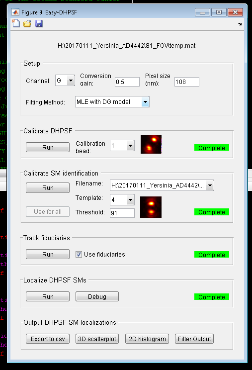
    1. Initialize Easy-DHPSF software in MATLAB. Under Setup, set Channel to G and set Fitting Method to MLE with DG model. G refers to the green channel camera, as the fluorescent protein being used for data acquisition emits with green wavelengths. MLE with DG Model refers to Maximum Likelihood Estimation with Double-Gaussian model.
       NOTE: The pixel size and conversion gain are dependent on the specific optical setup, and may need to be altered.
    2. Under the Calibrate DHPSF section, click Run. Click OK on the following pop-up window to keep default settings.
    3. Select the image stack saved in steps 1.13-1.14. Next, select the image stack with the dark background saved in step 1.15. Finally, select the .txt file that was automatically saved during step 1.14. This file contains the Z-position of the stage throughout the scanning process.
    4. In the next pop-up window, if the full camera chip was not used for the field of view, input the starting x0 and y0 positions on the chip. Otherwise, input x0 = 1 and y0 = 1.This information can be found in HCImage Live under the Binning and SubArrary section.
    5. In the following window, resize and reposition the box that appears over the image of the fluorescent beads so that it is approximately 100 x 100 pixels in size and centered over a single fluorescent DHPSF signal. Then, double-click to continue.
       NOTE: The chosen DHPSF should be isolated from the other DHPSF signals and ideally be the brightest bead possible.
    6. Click in the center of the DHPSF signal, in between the two lobes, then hit Enter. The following window shows a zoomed-in view of the chosen DHPSF. More precisely choose the location of the center of the DHPSF by clicking.
       NOTE: The program will then fit the DHPSF, and display the raw image and the reconstruction from the fit. It will also output template images from the Z calibration corresponding to a DHPSF cross section at different Z positions. These will be used later for fitting of the experimental data. The program will output the X,Y, and Z position estimated in each frame. In a well aligned optical system, X and Y should change very little (~30 nm deviation) as the Z position changes. If the output variation is larger than 30 nm, the phase mask, located in the Fourier plane of the imaging system (Figure 1), should be realigned and steps 1.9-1.16 repeated.
    7. Save the Easy-DHPSF GUI by clicking on the Save icon in the upper left corner of the GUI. This can later be loaded by clicking on the Load icon in the GUI.
       NOTE: The Z calibration procedure should be conducted on each day of an experiment to account for alignment changes in the microscope that may have occurred due to temperature fluctuations or mechanical vibrations.

2. Bacterial culture preparation

1. Prepare culture media supporting bacterial cell growth. For Y. enterocolitica, use 5 mL of BHI (Brain Heart Infusion) broth containing nalidixic acid (35 µg/mL) and 2,6-diaminopimelic acid (80 µg/mL). Here, a Y. enterocolitica strain is used that has the protein YscQ tagged with the fluorescent protein eYFP²³.
2. Inoculate media with bacterial cultures from freezer stocks or plate cultures.
3. Grow the culture at 28 °C with shaking overnight.
4. Dilute a small amount (~250 µL) of saturated overnight culture to 5 mL using fresh culture media.
5. Grow the culture at 28 °C with shaking for 60-90 min.
6. Induce expression of fluorescent fusion protein. For Y. enterocolitica, heat shock the cells to 37 °C in a water shaker to induce the yop regulon.
7. Incubate the cells for an additional 3 h at 37 °C with shaking.
8. Centrifuge 1 mL of culture at 5,000 x g for 3 min at room temperature. Discard the supernatant.
9. Wash the pellet 3 times with 1 mL of M2G media.
10. Re-suspend the pelleted bacteria in ~250 µL of M2G Media.
11. Add fluorescent beads as fiducial markers. Fluorescent bead solution should be added in appropriately diluted amounts, so that there are only 1-2 beads per FOV when viewed in the microscope.
12. Gently pipette or vortex the suspension to separate aggregated cells.
13. Plate 1.5 µL of suspension on a 1.5-2% agarose pad made with M2G.
14. Invert the agarose pad and place it on an ozone-cleaned microscope cover slip. The cover slip should be placed in an ozone cleaner for 30 min to reduce any inherent fluorescence background.

3. Data acquisition

1. Mount the sample cover glass onto the sample holder of an inverted fluorescence microscope and secure it in place using adhesive tape or spring loaded sample holder clips.
2. Add a drop of immersion oil onto the microscope objective, then place the sample holder onto microscope and secure it in place.
3. Initialize graphical user interface (GUI) to control the microscope’s camera, sample stage, and excitation lasers. Here, custom-written software in MATLAB is used for instrument control.
4. Initialize camera software HCImage Live. In the Capture tab under the Camera Control section, set the exposure time to 0.025 s. Click Live to begin a live feed of the camera.
5. Adjust the X and Y positions of the microscope stage by clicking the XY-Pos arrows under the Micro-Positioning Stage section of the GUI to scan around the sample and find a FOV with an appropriately dense population of bacterial cells.
   NOTE: To maximize data throughput, cells should be as dense as possible, without overlapping or touching cells. The FOV should also include at least 1 fluorescent bead to be used as a fiducial marker, preferably positioned in a corner of the FOV.
6. Adjust the Z position of the microscope stage by clicking the Z-Pos arrows under the Nano-Positioning Stage section of the GUI, so that the fluorescent bead’s DHPSF lobes are vertical.
7. Under Sequence | Scan Settings, change the number of frame counts to 20,000. Choose a save destination folder by clicking on the button labelled …. Finally click Start to collect up to 20,000 camera frames using a short exposure time of 0.025 s. eYFP photoblinking is initiated using high intensity excitation light at 514 nm^19,25.
   NOTE: Here, a laser intensity of ~350 W/cm² at the focal plane is used for initial bleaching and subsequent imaging of single EYFP molecules. Photoactivation of eYFP molecules at UV wavelengths during imaging was not used. There should be at most one single-molecule signal per bacterial cell. If the density of single-molecule signal is too high initially, continue to illuminate until sufficient photobleaching occurs before beginning data acquisition.
8. Turn off the laser illumination by clicking Close 515 nm laser in the GUI. Collect 200 frames of dark images using the same exposure time.
9. In the GUI, check the box next to Thorlabs LED and click Toggle Mirror Up. This will switch the pathway from the fluorescence pathway to the phase contrast pathway.
10. Initialize the data acquisition software IC Capture 2.4. This controls the camera in the phase contrast pathway. Press the Start/Stop Live Display button to view a live feed from the camera. Click Capture | Save Image to collect a phase contrast image of the cells in the field-of-view.
11. Repeat steps 3.5-3.10 for additional FOVs. Here, data acquired from ~500 bacterial cells in ten different FOVs is used to increase the number of single-molecule trajectories available for analysis.
    CAUTION: Cells mounted on the agarose pads for long periods of time may behave differently than freshly mounted cells. Additionally, the agarose pad may lose its integrity after some time, which may adversely affect data quality. Typically, at most 3 FOV (~30 min on the microscope) are used per sample slide.

4. Data processing

NOTE: A modified version of the Easy-DHPSF software²⁴ is used in MATLAB for the analysis of the raw camera frames to extract single-molecule localizations. Easy-DHPSF is used specifically to fit DHPSF localizations in single-molecule imaging. Custom changes were made to implement Maximum Likelihood Estimation (MLE)-based fitting routine that accounts for the pixel-dependent noise characteristics of modern sCMOS cameras²⁶. It was also modified to accept the image file type output from the HCImage Live program (.dcimg). For a more detailed explanation of the software and the individual steps, please see Lew et al.²⁴

1. Initialize the Easy-DHPSF GUI in MATLAB (Supplementary Figure 2). Load in the file saved in step 1.16.8.
2. Determining threshold values for each of the 7 templates output in step 1.16.7
   1. Under the Calibrate SM identification section, click Run. Click OK on the following two pop-up windows to keep default settings.
   2. Open the image stack containing the data from the first FOV when prompted.
   3. Choose a small range of frames to match templates. Typically frames 1001-2000 are used to avoid dense overlapping signals in the first several hundred frames. Click OK on the following pop-up window to keep default settings. Click Cancel when prompted for the sequence log file in the following window.
   4. Open the image stack with the dark background saved in step 3.8. Click ‘OK’ in the following pop-up window to leave the parameters for the background estimation set to default. The default is to estimate the background using a median filter²⁷ covering 100 subsequent camera frames around the current frame.
   5. In the next window, resize the box overlaid on the image to cover the full FOV, then double-click to continue.
   6. Define the region of interest by clicking several points on the image to create a polygon. The region of interest should include as much of the field of view as possible, while ensuring that any fluorescent beads (very bright objects) in the image do not lay within the polygon, then double-click to continue.
      NOTE: The software will then attempt to match the templates to the image, and will display an image with possible matches circled.
   7. When the software has stopped, it will save many images of found template matches and display the corresponding threshold value in a pre-defined folder. A higher threshold value corresponds to a better match. For each template number, examine the example matches and determine the lowest threshold that exhibits an image of a DHPSF. Input these thresholds for each of the 7 templates under the Calibrate SM Identification section in the Easy-DHPSF GUI.
      NOTE: The program will attempt to automatically choose and input thresholds, however, these are often unreliable and should be manually checked. Thresholds are chosen such that few true single-molecule signals are missed, but the number of false positive candidates for fitting remains computationally manageable.
   8. Save the Easy-DHPSF GUI again by clicking on the Save icon in the upper left corner.
3. Fitting the fluorescent bead in the FOV to use as a fiducial marker
   1. Under the Track fiduciaries section of the Easy-DHPSF GUI, click Run. Click OK on the following two pop-up windows to keep default settings.
   2. Drag the box overlaid on the image and center it over the DHPSF signal from the fluorescent bead, then double-click.
   3. Click in the center of the DHPSF signal, at the midpoint between the two lobes, then hit enter. Click Cancel when prompted for the sequence log file in the following window.
      NOTE: The software will fit the DHPSF in all camera frames, and display the raw image and the reconstructed image. When the software has finished, it will output figures with X,Y, and Z positions of the fluorescent bead over the duration of the image acquisition.
   4. Check the box next to Use fiduciaries and save the Easy-DHPSF GUI again by clicking on the Save icon in the upper left corner.
4. Find and fit all localizations in all camera frames using the template thresholds obtained in step 4.2.
   1. Under the Localize DHPSF SMs section of the Easy-DHPSF GUI, click Run. Click OK on the following pop-up windows to keep default settings. Click Cancel when prompted for the sequence log file in the following window.
      NOTE: The software will find and fit the DHPSF using a double-Gaussian model if the quality of the match is above the user-defined threshold. It will display the raw image with circles around template matches as well as an image of the reconstructed DHPSF fits.
   2. Save the Easy-DHPSF GUI again by clicking on the Save icon in the upper left corner.
5. Viewing single-molecule localizations and filtering out unwanted or unreliable localizations
   1. Under the Output DHPSF SM localizations section, click Filter Output.
   2. Click OK in the following three windows to perform an interpolation of the fiducial X,Y, and Z positions over time. In most cases, the default options are sufficient. If the black interpolated line does not reflect a reasonable interpolation of the red position line, change the interpolation parameters in the pop-up window.
      NOTE: The interpolated line is used for stage-drift correcting the single-molecule localizations.
   3. Open the corresponding phase contrast image for the FOV being analyzed when prompted. Click OK on the following two pop-up windows to keep default settings.
   4. In the following two pop-up windows, change the filter values to allow for more strict or more lenient single-molecule localization requirements, then click OK.
   5. In the window that appears, drag or resize the box overlaid on the images to view the desired region of interest and double-click to continue.
   6. A 3D reconstruction of single-molecule localizations is displayed. Use the figure tools to manipulate the reconstruction (rotate, zoom, etc). Click Continue to display another dialogue box asking ‘Would you like to replot with a different parameter set?’. If the results are satisfactory, click No. If they are not, click Yes.
      NOTE: Common reasons for unsatisfactory results include the phase contrast image not being correctly overlaid with the localization data or the initial template thresholds were too low creating many false positive localizations. If Yes was selected, the software will return to step 4.5.4 so that new parameter values can be defined. If No was selected, the results will be saved.

5. Data post-processing

1. Using custom-written software in MATLAB, crop the phase contrast image so that only the region that contains cells that were imaged under the fluorescence microscope remains. This step is necessary because the phase contrast image covers an area much larger than the fluorescence image. Cropping the image simplifies the next step.
2. Segment individual cells by processing the phase contrast image with the OUFTI²⁸ software (Supplementary Figure 3)
   1. Initialize OUFTI in MATLAB. Load the cropped phase contrast image from previous step by clicking on Load phase.
   2. Click File to choose and name a save location for the output file.
   3. Select Independent frames under the Detection and Analysis heading.
   4. Click Load Parameters to load parameters for cell detection. Examples of parameters include acceptable cell area, cell width and a cell splitting threshold.
      NOTE: All of these parameters should be adjusted to maximize performance for the specific cell sizes and image quality being used. Importantly, the algorithm parameter should be set to subpixel to allow for precise measurement of cell outlines.
   5. Click This frame to begin cell segmentation. Cell outlines will appear over the phase contrast image when the process is finished.
   6. Using the controls under the Manual section, split cells, add cells, or refine cell outlines to obtain outlines for cells that were inaccurately segmented during the automated process.
   7. Output the cell outlines by clicking Save analysis.
3. Use custom-written software in MATLAB to precisely overlay the outlines obtained in the previous step with the single-molecule localizations. The following substeps detail the steps of the software.
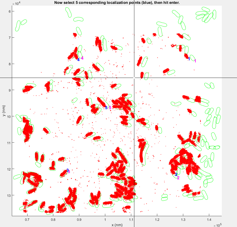
   1. Manually select 5 control point pairs in the pop-up window by roughly estimating and clicking on the position of the cell poles of the same five cells in both the single-molecule localization data and cell outlines, generated in the previous step. The position of the cell pole can be roughly estimated by mentally drawing a convex hull around the single-molecule localizations belonging to one cell and selecting the point of highest curvature (Supplementary Figure 4).
   2. Generate a 2D affine transformation function using the cp2tform function in MATLAB and use it to generate a rough overlay of the cell outlines and the single-molecule localizations.
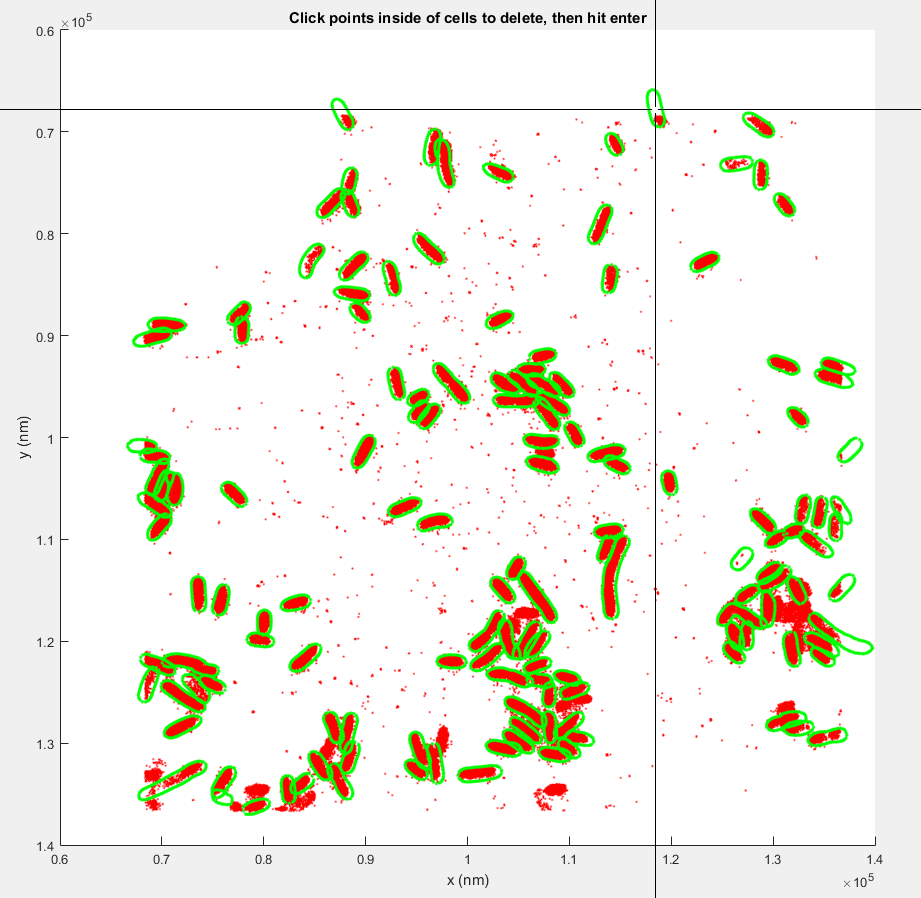
   3. Delete cells containing fewer than 10 localizations and remove cells that are positioned partially outside the field-of-view. Manually delete any additional unwanted cells in the pop-up window by clicking inside of their cell outline (Supplementary Figure 5).
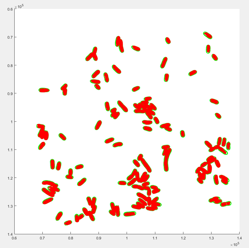
   4. Use the center of mass for all remaining cell outlines and single-molecule localizations within them to form a larger set of control point pairs, re-compute the 2D transformation function, and use it to generate a final overlay of the cell outlines and the single-molecule localizations.
   5. Assign localizations that reside within the boundary of a cells outline to that cell. Discard any localizations not located within any cell outline (Figure 2a, Supplementary Figure 6).

6. Single-molecule tracking

NOTE: The following section is completed using custom-written software in MATLAB. This section describes the steps the software performs.

1. For localizations assigned to the same cell and in subsequent camera frames, calculate the Euclidean distance between the localizations. If the distance between the localizations is below a threshold of 2.5 µm, link the localizations by assigning them to the same single-molecule trajectory.
   NOTE: It is important to only consider localizations within a single cell, so that localizations in adjacent cells that happen to meet the spatial and temporal threshold requirements are not linked. The 2.5 µm threshold was chosen as the maximum distance a very fast molecule (30 µm²/s) could travel in the length of the exposure time (0.025 s) plus a 20% buffer.
2. Discard trajectories shorter than 4 localizations. If two or more localizations (i.e., two or more fluorescing emitters) are simultaneously present in a cell, discard the associated trajectories. Setting the track length minimum to 4 localizations allows several distance measurements to be averaged yielding a more accurate estimate of the diffusion coefficients.
3. Calculate the mean squared displacement (MSD) for a given trajectory by:
   (1)
   where N is the total number of localizations in the trajectory and x_n is the position of the molecule at time point n.
4. Compute the apparent diffusion coefficient, D* by
   (2)
   where m = 2 or 3 is the dimensionality of the measurement and Δt is the camera exposure time.
   NOTE: A typical experiment will produce ~5,000-100,000 trajectories in total, resulting in an apparent diffusion coefficient distribution with that many counts.

7. Monte-Carlo simulation of Brownian motion in a confined volume

NOTE: Create libraries of simulated apparent diffusion coefficient distributions by performing Monte Carlo simulations of Brownian motion confined to a cylindrical volume, using 64 values in the range of 0.05–20 µm²/s as input parameters (software available from the authors upon request). This range was chosen to cover the range of previously estimated diffusion coefficients of fluorescent (fusion) proteins in bacteria. 64 diffusion coefficients are used to sample this range sufficiently. This section is performed using custom-written software in MATLAB and describes the steps the software automatically takes. The rod-shaped Y. enterocolitica cells used here are approximated by a cylindrical volume of length l = 5 µm and diameter d = 0.8 µm.

1. Initiate individual trajectories at a random position in the cylindrical volume, and simulate their random (i.e., Brownian) diffusion steps using a time interval of 100 ns (time interval should be much shorter than the camera exposure time to enable sufficient sampling of the position over the course of a camera frame). Sample each displacement step for an input D from the corresponding Gaussian distribution function by rearrangement of Eqn. 2 and add it to the previous position:
   (3)
   where the randn function in MATLAB samples a random number from a normal distribution. If a step causes the molecule to be displaced outside of the volume of the cylinder, reflect the molecule back inside the cylinder at a random angle.
2. For each time interval, generate a DHPSF image that corresponds to the instantaneous x,y,z position of the simulated emitter.
   1. To match experimental conditions, simulate images containing 1,000 photons per localization, with a laser background of 13 photons per pixel, and Poisson noise. In addition, add dark offset of ~50 photons per pixel and Gaussian read noise (σ ~1.5 photons), consistent with experimental camera calibration measurements. Finally, multiply the image by the experimentally measured pixel-dependent gain of the sCMOS camera to obtain the image in units of detector counts.
      NOTE: After these manipulations, the signal-to-noise ratio of the final image is ~2.
   2. Generate motion-blurred images that reflect the changing position of the molecules by summing 50 DHPSF images simulated during the exposure time used during experimental data acquisition. To limit computational expense, only 50 periodically sampled positions were chosen to generate an image (instead of all 250,000 positions sampled during a 0.025 s exposure time at a sampling interval of 100 ns).
      NOTE: The length (number of frames) of simulated trajectories should match the average length of experimental trajectories. In this case, the number of frames per trajectory is 6.
3. Generate 5,000 trajectories for each of the 64 simulated input diffusion coefficients.
4. Analyze simulated camera frames as described in the Data Processing section.
5. Link localizations into trajectories as described in the Single-Molecule Tracking section.
6. Interpolate the cumulative distribution function (CDF) for each simulated distribution using B-spline interpolation of order 25. Interpolated distributions are necessary so that they can be queried at arbitrary points.
7. Interpolate the resulting B-spline curves along the D-axis (D is the true unconfined diffusion coefficient that governs the motion of the simulated emitters) using the scatteredInterpolant function in MATLAB (specify the ‘natural’ interpolation method). This provides a continuous 2D function from which any apparent diffusion coefficient distribution corresponding to a true diffusion coefficient value in the range of 0.05-20 µm²/s can be queried.

8. Experimental apparent diffusion coefficient distribution fitting

NOTE: Fit experimentally measured distributions of apparent diffusion coefficients using linear combinations of the simulated distributions generated in the previous section (Monte-Carlo simulation of Brownian motion in a confined volume). This section is performed using custom-written software in MATLAB and describes the steps the software automatically takes. For more information and examples of application, please see Rocha et al.²⁹

1. Perform a constrained linear least-squares fit (using the lsqlin function in MATLAB) of the experimental CDF using a periodically sampled array of simulated CDFs from the library created in section 7. The output of this step is a parameter vector containing the diffusion coefficients and population fractions of prevalent diffusive states in the experimental distribution.
2. Combine diffusive states with diffusion coefficient values within 20% of each other into a single diffusive state by weight averaging based on relative population fraction. This is the starting parameter vector.
   NOTE: To reduce model complexity, the diffusive states with diffusion coefficients below 0.5 µm²/s can be held constant during all of the following steps.
3. Create arrays of trial fitting parameter vectors with different numbers of diffusive states, ranging from a single diffusive state to a user-defined maximum number of states.
   1. Using the starting parameter vector, combine adjacent diffusive states through weighted averaging and split diffusive states into two states with equal population fractions and diffusion coefficients 20% above and below the original value. Repeat for all state combination and splitting possibilities.
4. Use each trial fitting parameter vector to initialize a non-linear least square fitting of 5 separate subsets of the data (using the fmincon function in MATLAB). Determine the quality of the fit by finding the residual sum of squares between the fit and the distribution corresponding to the remaining subsets (data cross-validation).
5. Use the average residual sum of squares of the 5 separate fittings for each trial vector as the overall quality of fit, determine the trial vector with the best quality of fit for each number of diffusive states.
6. Determine the optimal number of states by identifying the trial vector for which adding an additional state does not result in at least a 5% improvement in the quality of the fit.
7. Use this trial vector to initialize the non-linear least squares fitting of the full data set.
8. Estimate error for the individual parameters by resampling the data by bootstrapping and refitting with the same trial vector.

Representative Results

Under the experimental conditions described here (20,000 frames, trajectory length minimum of 4 localizations) and depending on the expression levels of the fluorescently labeled fusion proteins, approximately 200-3,000 localizations yielding 10-150 trajectories can be generated per cell (Figure 2a,b). A large number of trajectories is necessary to produce a well-sampled distribution of apparent diffusion coefficients. The size of FOV collected here is ~55 x 55 µm, with 10 FOV collected per experiment. Therefore, to obtain >5,000 trajectories per experiment each FOV should contain at least 50 cells. Ideally, the cell population should be made as dense as possible, but without having cells touch each other. If the cell density is too high, then the presence of touching or overlapping cells makes it challenging to segment them successfully using OUFTI(²⁸), as described in Data Post Processing. Poor segmentation can lead to localizations and trajectories assigned incorrectly between cells.

Here, we present apparent diffusion coefficient data on the Y. enterocolitica Type 3 secretion protein YscQ, which we N-terminally labeled with the fluorescent protein eYFP. YscQ is a structural component of a membrane-spanning molecular machine, called the injectisome. The injectisome is comprised of over 20 different proteins, many of which are present in multiple copy numbers. Type 3 secretion injectisomes are broadly utilized by pathogenic gram-negative bacteria to deliver virulent effector proteins directly into host cell during infection. YscQ dynamically binds and unbinds to and from the cytosolic side of the injectisome. As a result, YscQ is also found freely diffusing in the cytosol. By applying the data acquisition, processing, and analysis protocol described above, we determined that unbound YscQ exists in at least 3 distinct diffusive states (Figure 3). These 3 diffusive states correspond to different homo- and hetero-oligomeric complexes of YscQ and other Type 3 secretion proteins²³.

Figure 1: Optical diagram of microscope pathways. The microscope has a pathway for detection of fluorescence signal and a separate pathway for taking a phase contrast image. A motorized ‘flip-mirror’ is used to switch between the pathways. The camera detectors, excitation lasers, LED, and ‘flip-mirror’ are controlled remotely by computer. Please click here to view a larger version of this figure.

Figure 2: Single-molecule localizations and trajectories. (A). 3D single-molecule localizations of eYFP-YscQ in a Y. enterocolitica cell obtained in different frames (1,766 localizations). The localizations are overlaid on a phase contrast image of the cell. The green line indicates the cell outline based on the phase contrast image. (B). 3D single-molecule trajectories of eYFP-YscQ obtained from the localizations shown in panel A (142 trajectories). Different colors represent different single-molecule trajectories. Please click here to view a larger version of this figure.

Figure 3: Apparent diffusion coefficient distribution fitting of eYFP-YscQ in Y. enterocolitica. The apparent diffusion coefficient distribution for eYFP-YscQ in Y. enterocolitca was best fit with 3 diffusive states. Note that the probability density function (PDF) is shown here, while the data fitting was done by fitting the cumulative distribution function (CDF, Experimental Apparent Diffusion Coefficient Distribution Fitting). Figure adapted from Rocha et al²³. Please click here to view a larger version of this figure.

Supplementary Figure 1. Microscope Control GUI. The microscope GUI controls the micropositioner of the stage, excitation lasers, LED, and cameras for fluorescence emission. Please click here to download this file.

Supplementary Figure 2. Easy-DHPSF GUI. The Easy-DHPSF software is used to extract single-molecule localizations from the DHPSF signals. Please click here to download this file.

Supplementary Figure 3. Oufti Segmentation. The open source software OUFTI²⁸ is used to sement the cells. Here, the results of the cell segmentation are shown in green. Please click here to download this file.

Supplementary Figure 4. Selection of control points. Five points are selected in both the cell outline data and the localization data. The cell poles are used as reference points. These points are used to transform the data so that the cell outlines and localizations are correctly overlaid. Please click here to download this file.

Supplementary Figure 5. Delete unwanted cells. After the cell overlay, unwanted cells are manually deleted. Cells with unusually low/high amounts of localizations should be deleted, as well as any cells which are at the edge of the FOV. Please click here to download this file.

Supplementary Figure 6. Final overlay of cell outlines and localizations. After deletion of unwanted cells, the cell outlines and single-molecule localizations are finely transformed to get the final overlay. Localizations outside of cell outlines are deleted. Please click here to download this file.

Supplementary Mov. 1: Raw data for a single-molecule trajectory. Example of detection of eYFP-YscQ on the sCMOS camera. In frame 1, there is no fluorescence signal. In frames 2-10, fluorescence is detected from a single molecule. In each successive frame, the position and orientation of the DHPSF changes, indicating diffusion of this molecule. Finally, in frame 11, there is once again an absence in fluorescence signal, indicating the end of the trajectory. Each pixel is 108 x 108 nm. Please click here to download this file.

Supplementary Mov. 2: Raw data for a missed single-molecule trajectory. Frames 1-3 show fluorescence signal for a single emitter. However, frames 4-6 show the presence of two overlapping DHPSFs, indicating the presence of two emitters in close proximity. In such cases, the individual DHPSFs may not be correctly fit because of their overlap. Even if both DHPSFs are successfully fit, any trajectory observed containing these localizations would be discarded. Two or more localizations in the same cell may lead to incorrect assignments of localizations to a given trajectory. Each pixel is 108 x 108 nm. Please click here to download this file.

Discussion

A critical factor for the successful application of the presented protocol is to ensure that single-molecule signals are well-separated from each other (i.e., they need to be sparse in space and in time (Supplementary Mov. 1)). If there is more than one fluorescing molecule in a cell at the same time, then localization could be incorrectly assigned to another molecules’ trajectory. This is referred to as the linking problem³⁰. Experimental conditions, such as protein expression levels and excitation laser intensity can be chosen to avoid the linking problem. However, care should be taken to obtain wild-type protein expression levels to ensure representative results. Here, we used allelic replacements under the control of the native promoters instead of chemically inducible expression, to ensure native expression levels of the labeled proteins. Thus, the excitation laser intensity (for eYFP blinking) or the activation laser intensity (for photo-activatable fluorescent probes) can be used to control the concentration of active emitters in time. Alternatively, when chemical dye labeling is used in conjunction with HALO and SNAP tags^31,32, then the dye concentration can be reduced until fluorescent signals are sparse enough to track single molecules³³. The protocol presented here further eliminates the linking problem by discarding any trajectories for which two or more localizations are simultaneously present in the same cell (Supplementary Mov. 2). Thus, if single-molecule signals are too dense, a large amount of  data is automatically discarded during processing. Under the excitation conditions used here (λ_ex = 514 nm at 350 W/cm²), we obtained 10-150 trajectories per bacterial cell when acquiring 20,000 frames over the course of 8 min. On the other hand, if experimental conditions are chosen such that single-molecule signals are sparse, then the data acquisition throughput may be low, so that obtaining a sufficiently large number of single-molecule trajectories would require imaging additional cells in additional fields-of-view. Acquiring a large number of trajectories is beneficial, because the errors in the fitted parameters (the diffusion coefficients and the population fractions) decrease as the number of trajectories that are analyzed increase²⁹.

Achieving large numbers of single-molecule trajectories requires high data-acquisition throughput. As a wide-field technique, single-molecule localization microscopy acquires data for each cell in the FOV simultaneously, and researchers have begun to take advantage of new sCMOS detectors that afford large FOVs^26,34,35. However, excitation laser powers of several Watts are required to achieve uniform intensities sufficient for single-molecule localization microscopy throughout such large FOVs. Such laser powers may be above the damage threshold of commercially available objective lenses. Lenslet arrays employed to make the excitation laser intensities uniform in large FOVs may be able to circumvent this issue³⁴. Additionally, optical aberrations become pronounced when imaging far away from the optical axis. As a result, the shape of the DHPSF may become too distorted to be successfully fit by a double Gaussian model employed in easy DHPSF. When imaging in an ultrawide FOV, more sophisticated spatially-varying PSF models are required³⁶. To avoid these complicating factors, the data presented here were acquired in a relatively small FOV (diameter = 55 µm) and data from 10 FOVs were pooled to obtain more than 75,000 single-molecule trajectories.

Fitting of the experimentally measured apparent diffusion coefficient distributions with simulated distributions requires realistic simulation of the experimental data. Static and dynamic localization errors in camera-based tracking can affect the quality of the measurement^11,13. Static localization errors are due to the finite numbers of photons collected per fluorescence emitter, which results in an imprecise PSF shape and thus result in single-molecule localizations of limited precision^2,37,38. Dynamic localization errors arise due to moving emitters that generate blurred PSFs³⁹. When an algorithm is applied to fit the shape of the PSF, motion-blurred images provide localizations with limited accuracy and precision³⁹. In severe cases of rapid molecule movement, the image may be too distorted to fit, resulting in an unsuccessful fit and thus no recorded localization. Simulating spatially blurred PSFs with realistic signal to-noise ratios and localizing with the same fitting algorithm as experimental data accounts for both static and dynamic localization error. Second, rapidly diffusing molecules can be strongly confined to small volumes, such as the cytosol of a bacterial cell. As a result, the apparent diffusion coefficients are smaller, on average, than those expected for unconfined motion. Spatial confinement results in an overall left-shift of the distribution towards smaller diffusive values. Importantly, the shape of the distribution is no longer expressible as an analytical function. By explicitly accounting for static and dynamic localization errors due to motion blurring and confinement effects through stochastic simulations, realistic distributions can be obtained²³.

The described diffusion analysis relies on two key assumptions regarding the dynamic behavior of the molecules in the biological environment. It assumes that diffusive states are described by confined Brownian motion and that they do not interconvert on the timescale of a single-molecule trajectory. We have experimentally verified that the assumption of confined Brownian motion is justified for free eYFP diffusion in Y. enterocolitica²³. These results are in agreement with a number of studies in various bacterial species that have established that the motion of cytosolic proteins, fusion proteins, and biomolecular complexes smaller than 30 nm can be described by Brownian motion^{18,40,41,42,43,44,45}. Non-specific collisions of small fluorescently labeled proteins with other cellular components may slow down the diffusion rates,^45,46 but do not lead to deviations from Brownian diffusion. By contrast, specific interaction with cognate binding partners can produce a change in the diffusion coefficient, as recently shown for the Y. enterocolitica Type 3 secretion protein YscQ²³. The validity of the second assumption is difficult to assess, especially for systems for which neither the diffusive states nor the binding kinetics are known. The situation is further complicated because any oligomerization states and binding kinetics measured in vitro, may not reflect the structures and dynamics that occur in vivo. A recent theoretical study based on the analysis framework presented here suggests that it may be possible to extract the state switching kinetics in addition to the diffusion coefficients and population fractions²⁹.

In summary, we present an integrated protocol for resolving the diffusive states of fluorescently labeled molecules based on single-molecule trajectories measured in living bacterial cells. As presented here, the protocol is applied to 3D single-molecule localization microscopy using the double-helix PSF for imaging in Y. enterocolitica, a bacterial pathogen. However, with only a few modifications, the protocol can be applied to any type of 2D or 3D single-molecule localization microscopy and specimen geometry.

Materials

Name	Company	Catalog Number	Comments
2,6-diaminopimelic acid	Chem Impex International	5411	Necessary for growth of Y. enterocolitica cells used.
4f lenses	Thorlabs	AC508-080-A	f = 80mm, 2"
514 nm laser	Coherent	Genesis MX514 MTM	Use for fluorescence excitation
agarose	Inivtrogen	16520100	Used to make gel pads to mount liquid bacterial sample on microscope.
ammonium chloride	Sigma Aldrich	A9434	M2G ingredient.
bandpass filter	Chroma	ET510/bp	Excitation pathway.
Brain Heart Infusion	Sigma Aldrich	53286	Growth media for Y. enterocolitica.
calcium chloride	Sigma Aldrich	223506	M2G ingredient.
camera	Imaging Source	DMK 23UP031	Camera for phase contrast imaging.
dielectric phase mask	Double Helix, LLC	N/A	Produces DHPSF signal.
disodium phosphate	Sigma Aldrich	795410	M2G ingredient.
ethylenediaminetetraacetic acid	Fisher Scientific	S311-100	Chelates Ca2+. Induces secretion in the T3SS.
flip mirror	Newport	8892-K	Allows for switching between fluorescence and phase contrast pathways.
fluospheres	Invitrogen	F8792	Fluorescent beads. 540/560 exication and emission wavelengths. 40 nm diameter.
glass cover slip	VWR	16004-302	#1.5, 22mmx22mm
glucose	Chem Impex International	811	M2G ingredient.
immersion oil	Olympus	Z-81025	Placed on objective lens.
iron(II) sulfate	Sigma Aldrich	F0518	M2G ingredient.
long pass filter	Semrock	LP02-514RU-25	Emission pathway.
magnesium sulfate	Fisher Scientific	S25414A	M2G ingredient.
microscope platform	Mad City Labs	custom	Platform for inverted microscope.
nalidixic acid	Sigma Aldrich	N4382	Y. enterocolitica cells used are resistant to nalidixic acid.
objective lens	Olympus	1-U2B991	60X, 1.4 NA
Ozone cleaner	Novascan	PSD-UV4	Used to eliminate background fluorescence on glass cover slips.
potassium phosphate	Sigma Aldrich	795488	M2G ingredient.
Red LED	Thorlabs	M625L3	Illuminates sample for phase contrast imaging. 625nm.
sCMOS camera	Hamamatsu	ORCA-Flash 4.0 V2	Camera for fluorescence imaging.
short pass filter	Chroma	ET700SP-2P8	Emission pathway.
Tube lens	Thorlabs	AC508-180-A	f=180 mm, 2"
Yersinia enterocolitica dHOPEMTasd	N/A	N/A	Strain AD4442, eYFP-YscQ
zero-order quarter-wave plate	Thorlabs	WPQ05M-514	Excitation pathway.

References

- Kapanidis, A. N., Uphoff, S., Stracy, M. Understanding Protein Mobility in Bacteria by Tracking Single Molecules. Journal of Molecular Biology. , (2018).
- Betzig, E., et al. Imaging intracellular fluorescent proteins at nanometer resolution. Science. 313 (5793), 1642-1645 (2006).
- Hess, S. T., Girirajan, T. P. K., Mason, M. D. Ultra-high resolution imaging by fluorescence photoactivation localization microscopy. Biophysical Journal. 91 (11), 4258-4272 (2006).
- Rust, M. J., Bates, M., Zhuang, X. W. Sub-diffraction-limit imaging by stochastic optical reconstruction microscopy (STORM). Nature Methods. 3 (10), 793-795 (2006).
- Chen, T. Y., et al. Quantifying Multistate Cytoplasmic Molecular Diffusion in Bacterial Cells via Inverse Transform of Confined Displacement Distribution. Journal of Physical Chemistry B. 119 (45), 14451-14459 (2015).
- Mohapatra, S., Choi, H., Ge, X., Sanyal, S., Weisshaar, J. C. Spatial Distribution and Ribosome-Binding Dynamics of EF-P in Live Escherichia coli. mBio. 8 (3), (2017).
- Stracy, M., et al. Single-molecule imaging of UvrA and UvrB recruitment to DNA lesions in living Escherichia coli. Nature Communications. 7, 12568 (2016).
- Persson, F., Lindén, M., Unoson, C., Elf, J. Extracting intracellular diffusive states and transition rates from single-molecule tracking data. Nature Methods. 10 (3), 265-269 (2013).
- Bakshi, S., Choi, H., Weisshaar, J. C. The spatial biology of transcription and translation in rapidly growing Escherichia coli. Frontiers in Microbiology. 6, 636 (2015).
- Mustafi, M., Weisshaar, J. C. Simultaneous Binding of Multiple EF-Tu Copies to Translating Ribosomes in Live Escherichia coli. mBio. 9 (1), (2018).
- Michalet, X., Berglund, A. J. Optimal diffusion coefficient estimation in single-particle tracking. Physical Review E. 85 (6), (2012).
- Michalet, X. Mean square displacement analysis of single-particle trajectories with localization error: Brownian motion in an isotropic medium. Physical Review E Statistical, Nonlinear, and Soft Matter Physics. 82 (4 Pt 1), 041914 (2010).
- Backlund, M. P., Joyner, R., Moerner, W. E. Chromosomal locus tracking with proper accounting of static and dynamic errors. Physical Review E Statistical, Nonlinear, and Soft Matter Physics. 91 (6), 062716 (2015).
- Stracy, M., et al. Live-cell superresolution microscopy reveals the organization of RNA polymerase in the bacterial nucleoid. Proceedings of the National Academy of Sciences of the United States of America. 112 (32), E4390-E4399 (2015).
- Plochowietz, A., Farrell, I., Smilansky, Z., Cooperman, B. S., Kapanidis, A. N. In vivo single-RNA tracking shows that most tRNA diffuses freely in live bacteria. Nucleic Acids Research. 45 (2), 926-937 (2017).
- Koo, P. K., Mochrie, S. G. Systems-level approach to uncovering diffusive states and their transitions from single-particle trajectories. Physical Review E. 94 (5-1), 052412 (2016).
- Uphoff, S., Reyes-Lamothe, R., Garza de Leon, F., Sherratt, D. J., Kapanidis, A. N. Single-molecule DNA repair in live bacteria. Proceedings of the National Academy of Sciences of the United States of America. 110 (20), 8063-8068 (2013).
- Bakshi, S., Bratton, B. P., Weisshaar, J. C. Subdiffraction-Limit Study of Kaede Diffusion and Spatial Distribution in Live Escherichia coli. Biophysical Journal. 101 (10), 2535-2544 (2011).
- Bakshi, S., Siryaporn, A., Goulian, M., Weisshaar, J. C. Superresolution imaging of ribosomes and RNA polymerase in live Escherichia coli cells. Molecular Microbiology. 85 (1), 21-38 (2012).
- Uphoff, S., Sherratt, D. J., Kapanidis, A. N. Visualizing Protein-DNA Interactions in Live Bacterial Cells Using Photoactivated Single-molecule Tracking. JoVE. (85), e51177 (2014).
- Pavani, S. R. P., Piestun, R. Three dimensional tracking of fluorescent microparticles using a photon-limited double-helix response system. Optics Express. 16 (26), 22048-22057 (2008).
- Pavani, S. R. P., et al. Three-dimensional, single-molecule fluorescence imaging beyond the diffraction limit by using a double-helix point spread function. Proceedings of the National Academy of Sciences of the United States of America. 106 (9), 2995-2999 (2009).
- Rocha, J. M., et al. Single-molecule tracking in live Yersinia enterocolitica reveals distinct cytosolic complexes of injectisome subunits. Integrative Biology. 10 (9), 502-515 (2018).
- Lew, M. D., von Diezmann, A. R. S., Moerner, W. E. Easy-DHPSF open-source software for three-dimensional localization of single molecules with precision beyond the optical diffraction limit. Protocol Exchange. , (2013).
- Biteen, J. S., et al. Super-resolution imaging in live Caulobacter crescentus cells using photoswitchable EYFP. Nature Methods. 5 (11), 947-949 (2008).
- Huang, F., et al. Video-rate nanoscopy using sCMOS camera-specific single-molecule localization algorithms. Nature Methods. 10 (7), 653-658 (2013).
- Hoogendoorn, E., et al. The fidelity of stochastic single-molecule super-resolution reconstructions critically depends upon robust background estimation. Scientific Reports. 4, 3854 (2014).
- Paintdakhi, A., et al. Oufti: An integrated software package for high-accuracy, high-throughput quantitative microscopy analysis. Molecular microbiology. 99 (4), 767-777 (2016).
- Rocha, J. M., Corbitt, J., Yan, T., Richardson, C., Gahlmann, A. Resolving Cytosolic Diffusive States in Bacteria by Single-Molecule Tracking. bioRxiv. , 483321 (2018).
- Lee, A., Tsekouras, K., Calderon, C., Bustamante, C., Presse, S. Unraveling the Thousand Word Picture: An Introduction to Super-Resolution Data Analysis. Chemical Reviews. 117 (11), 7276-7330 (2017).
- Los, G. V., et al. HaloTag: A Novel Protein Labeling Technology for Cell Imaging and Protein Analysis. ACS Chemical Biology. , (2008).
- Gautier, A., et al. An Engineered Protein Tag for Multiprotein Labeling in Living Cells. Chemistry & Biology. 15 (2), 128-136 (2008).
- Bisson-Filho, A. W., et al. Treadmilling by FtsZ filaments drives peptidoglycan synthesis and bacterial cell division. Science. 355 (6326), 739-743 (2017).
- Douglass, K. M., Sieben, C., Archetti, A., Lambert, A., Manley, S. Super-resolution imaging of multiple cells by optimised flat-field epi-illumination. Nature Photonics. 10 (11), 705-708 (2016).
- Zhao, Z., Xin, B., Li, L., Huang, Z. L. High-power homogeneous illumination for super-resolution localization microscopy with large field-of-view. Optics Express. 25 (12), 13382-13395 (2017).
- Yan, T., Richardson, C. J., Zhang, M., Gahlmann, A. Computational Correction of Spatially-Variant Optical Aberrations in 3D Single Molecule Localization Microscopy. bioRxiv. , 504712 (2018).
- Gahlmann, A., Moerner, W. E. Exploring bacterial cell biology with single-molecule tracking and super-resolution imaging. Nature Reviews Microbiology. 12 (1), 9-22 (2014).
- Liu, Z., Lavis, L. D., Betzig, E. Imaging live-cell dynamics and structure at the single-molecule level. Mol Cell. 58 (4), 644-659 (2015).
- Berglund, A. J.
- Parry, B. R., et al. The bacterial cytoplasm has glass-like properties and is fluidized by metabolic activity. Cell. 156 (1-2), 183-194 (2014).
- English, B. P., et al. Single-molecule investigations of the stringent response machinery in living bacterial cells. Proceedings of the National Academy of Sciences of the United States of America. 108 (31), E365-E373 (2011).
- Niu, L. L., Yu, J. Investigating intracellular dynamics of FtsZ cytoskeleton with photoactivation single-molecule tracking. Biophysical Journal. 95 (4), 2009-2016 (2008).
- Coquel, A. S., et al. Localization of protein aggregation in Escherichia coli is governed by diffusion and nucleoid macromolecular crowding effect. PLoS Computational Biology. 9 (4), e1003038 (2013).
- Nenninger, A., Mastroianni, G., Mullineaux, C. W. Size Dependence of Protein Diffusion in the Cytoplasm of Escherichia coli. Journal of Bacteriology. 192 (18), 4535-4540 (2010).
- Dix, J. A., Verkman, A. S. Crowding effects on diffusion in solutions and cells. Annual Review of Biophysics. 37, 247-263 (2008).
- Elliott, L. C., Barhoum, M., Harris, J. M., Bohn, P. W. Trajectory analysis of single molecules exhibiting non-brownian motion. Physical Chemistry Chemical Physics. 13 (10), 4326-4334 (2011).